21st Friday Fun Session – 9th Jun 2017
Maximum subarray finds the contiguous subarray within a one-dimensional array having the largest sum.
Visualizing the divide and conquer solution
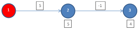
For the time being, let us forget about maximum subarray problem and focus on the divide and conquer solution that we discussed in the previous session.
If we visualize the tree, we see that from the left subtree the smallest value is propagated upwards. On the way up, it is treated as the buy value and the right side values are treated as sell values. This way profits are calculated and maximum among them is retained. So we see two themes of processing as we go from left to right of the array:
- Retain the minimum value and treat it as the buy value.
- Calculate profit by treating each value seen as we go right and retain the maximum profit.
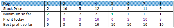
The above table shows day number in first row and the corresponding stock prices in second row. Third row shows the minimum value seen so far. The fourth row shows the profit had we sold on this day, buy price being the minimum value seen so far (shown in green).
The intuition
The intuition being, when we see a new lower value than the one already seen, we treat that as the new buy value. For example, when we see the new lower value 1 on day 5, onward we treat that as the new buy value and calculate profits considering each of the following days as sell days. This is because the new lower value (lowest till now) would give a better profit when the following days are treated as potential sell days. By treating the previous lower value 2 that was found on day 1, we already considered all possible profits prior to 5th day and retained the best among them. On 5th day, the utility of the previous lower value, which is 2, stops.
From divide and conquer to dynamic programming
Now let us now consider the dynamic programming (DP) point of view. In dynamic programming we make use of the result of an already solved overlapping subproblem.
On the first day, we can buy but cannot sell. After all, no profit would be made selling on the first day with the same price as the buy price. Also note that we have to buy and only then we can sell. So on day 1, profit is 0. Now if we want to find the best profit on day 2, can we use the solution of the previously solved overlapping subproblem? What is that already solved overlapping subproblem at day 2? Well, it is the best profit found for day 1, which is 0. How can we make use of the previous solution to find the best profit at day 2? Well, we have to consider two things:
- If we have to make the most profit by selling today, then we have to buy using the lowest price seen so far.
- If the profit calculated above is better than the best seen on previous day, then this is the new best. Else previous day’s best is still the best for today.
For example, on day 2 we realize that we can make a profit of (8-0) = 8 and it is better than the profit at day 1, which is 0. Hence, the best profit for day 2 is updated to 8. On day 3, we find we can make a profit of 3 but the best profit till day 2 is better than this. So, we retain day 2’s best profit as day 3 best profit.
So we realize, what we found by visualizing and transforming the divide and conquer solution is nothing but this dynamic programming. In fact, this is possibly one of the simplest forms of dynamic programming.
The below code would find the solution. For brevity buy day and sell day is not tracked that is easy to accommodate.
void StockDpN(double price[], int n, double &maxProfit)
{
  double minPriceSoFar = price[0];
  maxProfit = 0;

  for(int i=1; i<n; i++)
  {
    if(price[i] - minPriceSoFar > maxProfit)
      maxProfit = price[i] - minPriceSoFar;

    if(price[i] < minPriceSoFar)
     minPriceSoFar = price[i];
  }
}
The reverse can also be used. If we start from right and move leftwards, we have to keep track of the maximum value seen so far and that is the sell value. As we go left, we see new values and they are buy values. The associated code is not shown here.
Moving to maximum subarray problem
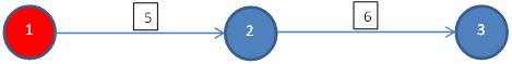
Suppose we buy a stock at one day and then sell it on the following day. For example, buy at day 1 and then sell on day 2. Buy at day 2 and then sell on day 3 and so on. Each day we make a profit, incur a loss and sometimes it is neutral, meaning no profit or loss (buy value and sell value being the same). The third row of the below table shows the same (loss shown in red).
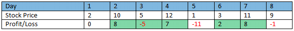
The optimal solution to our stock profit problem with our example set is to buy on day 1 at price 2 and sell it on day 4 at price 12, thus making a profit of 10. It is the same as saying:
- We buy at day 1 and sell at day 2 making profit 8 and then
- Buy at day 2 and sell at day 3 making loss 5 and then
- Buy at 3 and sell at day 4 making profit 7 and then
- Add all profits/losses made in our buy/sell operations that started by buying on day 1 and ended by selling on day 4. The final and best profit is: 8 + (-5) + 7 = 10.
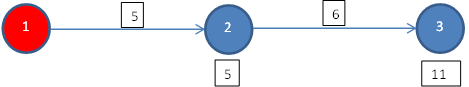
Thus we have transformed the previous stock profit problem to a maximum subarray problem. As explained earlier, we are interested to find contiguous portion of array that gives the maximum sum. In the above 8 values that we have, we got two such subarrays each giving a sum of 10. They are showed in colored boxes.
Kadane’s algorithm
Kadane’s algorithm also deploys DP to solve this. Once again in DP, we have to make use of already solved overlapping subproblems. Here it is done by this way:
- Maximum subarray ending in position i+1 includes already solved maximum subarray ending at i, if doing so increases the sum for subarray ending at i+1
- Else maximum subarray ending in position i+1 will only have itself.

Maximum subarray at day 1: day 1 value which is 0.
Maximum subarray at day 2: since adding the subarray sum for day 1, which is 0, is not increasing the sum for day 2, maximum subarray at day 2 will have only day 2 value itself, meaning 8.
Maximum subarray at day 3: subarray sum at day 2 is positive, which is 8, and helping day 3, so subarray at day 3 includes day 2. Subarray sum at day 3 = 8 + (-5) = 3.
It boils down to a simple thing. If the previous sum is positive then take it forward else not. The red color in the Maximum subarray sum row (4th row) shows the cases where it does not include the (immediately) prior subarray. In two cases it happens (8 at day 2 and 2 at day 6) because the prior sums (0 and -1 respectively) are not more than zero.
The code shown below implements this. Note that the input array profit contains the profit and loss unlike the earlier DP function where we passed the stock prices. It is also noteworthy that if all values are positive then the whole array is the maximum subarray. After all, adding all of them would give the highest sum.
void StockKadaneDpN(double profit[], int n, double &maxProfit)
{
  double curProfit = 0; maxProfit = 0;

  for(int i=1; i<n; i++)
  {
    curProfit = curProfit > 0 ? curProfit + profit[i] : profit[i];
    if(curProfit > maxProfit)
      maxProfit = curProfit;
  }
}
If we observe closely, we see that this DP is essentially the same as the one we discussed earlier in this post.
Backtrace
At the end, when we find the maximum subarray sum 10 at day 4, we will do what is called backtrace, typical of DP to find the path, in this case, the maximum subarray. We know that at day 4, we included the subarray ending at day 3. At day 3, we included the subarray ending at day 2. At day 2, we did not include prior subarray. So the maximum subarray starts at day 2 and ends at day 4. It could be easily tracked/stored as we went ahead in the computation using appropriate data structure and would not require a come back.
Map maximum subarray solution to stock profit
If we want to map this solution back to our stock profit problem, then we know the profit at start day of the maximum subarray, that is day 2, is essentially found by buying stock at the previous day that is day 1. So the solution is: buy at day 1 and sell at the last day of the maximum subarray that is day 4. And the profit would be the maximum subarray sum that is 10.
The transformations
This is an interesting problem to observe as we started with a O(n^2) brute force accumulator pattern, moved to O(n log n) divide and conquer that we optimized later to O(n). Finally, we transformed that to a O(n) DP solution only to find that it is interchangeable to O(n) maximum subarray problem that is also a DP solution.
Can we do better than O(n)? Well, that is not possible. After all, we cannot decide the best solution unless we read all the data at least once. Reading the data once is already O(n).
Where is pattern recognition here?
Maximum subarray essentially gives the brightest spot in a one-dimensional array. Finding this brightest spot is one kind of pattern recognition. Note that we just solved a problem that reads like this: given the profit/ loss made by a company over the period find the longest duration(s) when the company performed the best. The answer here is: from day 2 to day 4 or from day 6 to day 7.
Even though we focused on finding the single brightest spot, it is also possible to find, k brightest spots.
Again, maximum subarray considers only one dimension. In real life, data sets typically contain more than one dimension. For example, a problem involving two dimensions might read like: can you find the largest segment of the customers buying product x based on age and income? A potential answer might be: customer from age 30 to 40 years with income range $3000 – $6000. There are other algorithms to deal with multi-dimensional data.
GitHub: Stock Profit Kadane Code