Johnson’s Algorithm

47th Friday Fun Session – 19th Jan 2018

We have seen why Dijkstra’s algorithm cannot work with negative edge and that we cannot trivially add a constant to each of the edge weights and make them non-negative to proceed further. It is where Johnson’s algorithm comes into play. It finds a special set of offset values to remove the negative edges (change the negative edge weights to non-negative edge weights) and now this transformed graph is all set to work with Dijkstra’s algorithm.

How Does Johnson’s Algorithm work?

Johnson’s algorithm starts with a graph having negative edge(s). Let’s go through it using an example as shown below.

1

Add a New Node

It then adds a new vertex, let’s call it s, with edges starting from it and ending to each of the vertices of the existing graph, each having a cost of 0, as we have done earlier.

2.png

Apply Bellman-Ford

Then it applies Bellman-Ford, a Single Source Shortest Path (SSSP) algorithm that can work with a graph having negative edge(s). We will use s as the source, and find shortest path from it to all other vertices.

We also need to check whether a negative cycle exists, something that Bellman-Ford can detect. If it exists then we cannot proceed further as we cannot find shortest path in a graph with negative cycle. In our example graph, there is no negative cycle.

We find d[s, 1] = 0, d[s, 2] = -30, and d[s, 3] = 0 as shown below, using this code where d[s, t] indicates the shortest path from s to t.

3.png

Adjust Original Edge Weights

Now using these shortest path costs, original edges will be updated using the formula: w’[u, v] = w[u, v] + d[s, u] – d[s, v]. Applying the same for the original 3 edges in the original graph, we find,

w’[1, 2] = w[1, 2] + d[s, 1] – d[s, 2] = 20 + 0 – (-30) = 50

w’[1, 3] = w[1, 3] + d[s, 1] – d[s, 3] = 40 + 0 – 0 = 40

w’[3, 2] = w[3, 2] + d[s, 3] – d[s, 2] = (-30) + 0 – (-30) = 0

Now that we have adjusted the original edge costs, the new (cost) adjusted graph (without s and associated edges) does not have any more negative edge. Let’s see how the cost adjusted graph looks like.

4

Apply Dijkstra

With this non-negative edge graph we can proceed with Dijkstra’s algorithm. For each shortest path found in this graph from u to v, we have to adjust back the cost by subtracting d[s, u] – d[s, v] from it.

Is the Shortest Path Still the Same?

We are adjusting edge cost to remove negative edge. That way, we are changing the graph to some extent. However, while doing so we must preserve certain things of it. What was the cheapest cost in the original graph must still remain the cheapest path in the transformed graph. Let’s first verify whether that is indeed the case.

We will first look at the original graph (before edge cost adjustment). Let’s take a certain source destination pair (1, 2). There are two paths to reach from vertex 1 to vertex 2.

The first one (original):

d1[1, 2]

= from vertex 1 to vertex 2 directly using edge 1->2

= 20.

The second one (original):

d2[1, 2]

= from vertex 1 to 3 and then from 3 to 2

= 40 + (-30)

= 10.

Now let’s see how the costs of the same two paths change in the new cost adjusted graph.

The first one (cost adjusted):

d’1[1, 2]

= from vertex 1 to vertex 2 directly using edge 1->2

= 50.

The second one (cost adjusted):

d’2[1, 2]

= from vertex 1 to 3 and then from 3 to 2

= 40 + 0

= 40.

We see both the path costs have increased by 30, a constant. So what was earlier the shortest from vertex 1 to vertex 2, in the original graph, which was the second path, using two edges: edge 1->3 and edge 3->2, still remains the shortest path in the cost adjusted graph.

So how did that happen? Let’s have a closer look as to how the path cost changes.

The first one (cost adjusted):

d’1[1, 2]

= w’[1, 2]

= w[1, 2] + d[s, 1] – d[s, 2]

= d1[1, 2]  + d[s, 1] – d[s, 2]

The second one (cost adjusted):

d’2[1, 2]

= w’[1, 3] + w’[3, 2]

= w[1, 3] + d[s, 1] – d[s, 3] + w[3, 2] + d[s, 3] – d[s, 2]

= w[1, 3] + d[s, 1] + w[3, 2] – d[s, 2]

= w[1, 3] + w[3, 2] + d[s, 1] – d[s, 2]

= d2[1, 2] + d[s, 1] – d[s, 2]

So we see both the paths, with a certain source u and a certain destination v, have increased with a constant cost = d[s, u] – d[s, v], where s is the extra node that we added before applying Bellman-Ford algorithm.

We can easily find, no matter how many paths are present between a certain source s and a certain destination v, and no matter how many edges each of those paths uses, each of them would be adjusted by adding a constant cost = d[s, u] – d[s, v] to it. And hence, the shortest path in the original graph remains the shortest path in the new cost adjusted, non-negative edge graph.

Let’s consider a path that goes through 5 vertices: u, x1, x2, x3, and v.

In the cost adjusted graph the cost

d’[u, v]

= w’[u, x1] + w’[x1, x2] + w’[x2, x3] + w’[x3, v]

= w[u, x1] + d[s, u] – d[s, x1] + w[x1, x2] + d[s, x1] – d[s, x2] + w[x2, x3] + d[s, x2] – d[s, x3] + w[x3, v] + d[s, x3] – d[s, v]

= w[u, x1] + d[s, u] + w[x1, x2] + w[x2, x3] + w[x3, v] – d[s, v]

= w[u, x1] + w[x1, x2] + w[x2, x3] + w[x3, v] + d[s, u] – d[s, v]

= d[u, v] + d[s, u] – d[s, v]

By generalizing the above, we see that a constant cost d[s, u] – d[s, v] is getting added to all paths from u to v.

Are all Negative Edge Removed?

The second thing that we need to prove is: no longer there exists a negative edge in the adjusted graph. After applying Bellman-Ford, we computed the shortest paths from source s. Let’s assume, d[s, u] and d[s, v] are the shortest paths from s to any two vertices, u and v, respectively. In that case, we can say,

d[s, v] <= d[s, u] + w[u, v]

=> 0 <= d[s, u] + w[u, v] – d[s, v]

=> 0 <= w[u, v] + d[s, u] – d[s, v]

=> 0 <= w’[u, v]

We prove that the new edge cost, w’[u, v] is always non-negative.

Why Would We Use Johnson’s algorithm?

So here with Johnson’s algorithm, first we use Bellman-Ford to get a set of values; using which we transform the graph with negative edge to a graph with all non-negative edges so that we can apply Dijkstra’s algorithm.

But why would anyone want to do that? After all, both Bellman-Ford and Dijkstra are SSSP algorithms. What is the point of using one SSSP algorithm to transform a graph so that another SSSP algorithm can be used on the transformed graph?

Dijkstra’s Algorithm is Faster

Well, the reason being, the latter SSSP algorithm, namely Dijkstra’s, is much faster than Bellman-Ford. So, if we need to find shortest paths many times, then it is better that first we apply a bit more expensive SSSP alogorithm – Bellman-Ford to get the graph ready to work with Dijkstra’s algorithm. Then we execute much cheaper Dijkstra’s algorithm on this transformed graph, as many times as we want – later.

Sparse Graph

But in such a situation is it not better to run an ALL-Pairs Shortest Paths (APSP) algorithm like Floyd-Warshall? After all, Floyd-Warshall can compute APSP at a cost of O(V3) while Bellman-Ford costs O(|V| * |E|) that can shoot up to O(V3), when E=|V|2 for a dense graph.

Yes, that is correct. For a dense graph Johnson’s algorithm won’t possibly be useful. Johnson’s algorithm is preferable for a sparse graph when Bellman-Ford is reasonably efficient to work with it.

Index

Collation in MS SQL Server

53rd Friday Fun Session – 9th Mar 2018

What Does Collation Do in SQL Server?

Collation in SQL server does two things:

  1. Storage: specifies the character set/code page used to store non-Unicode data
  2. Compare and sort: determines how to compare and sort all textual data

No Bearing on Code Page of Unicode Data

Code page as specified in a collation is applicable only for non-Unicode characters. Unicode data is stored using UCS-2/UTF-16 character set (UCS-2 is a predecessor of UTF-16), code page 0, irrespective of what collation is in use. So collation has no bearing on the storage of nvarchar, nchar etc. type (Unicode) data.

Many Code Pages

Apart from code page 0 that is used for Unicode data, there are 16 other code pages for storing non-Unicode data.

SELECT
name,
COLLATIONPROPERTY(name, 'CodePage') AS [Code Page],
description
FROM ::fn_helpcollations()

Each of the around 3885 collations, as I can see in SQL Server 2012, uses one of these 17 code pages. As said, even when a collation uses one of those 16 non-Unicode code pages, for Unicode data (nvarchar etc.), code page 0 will always be used. Code page for Unicode data is not configurable. However, around 510 collations use code page 0. For them, even for non-Unicode data like varchar, code page 0 will be used.

Two Parts of a Collation Name

A collation name looks like SQL_Latin1_General_CP1_CI_AS. The first part indicates the (language and) code page. The later part CI, AS etc. indicates compare/sort rules.

No Bearing on Compare/Sort for Non-textual Data

Collation affects only textual data as far as comparing/sorting is concerned. Non-textual data like integer, date, bool, decimal etc. are not affected.

Options Associated with Collation

All the options as listed below dictate sorting preferences.

  1. Case-sensitive (_CS) – ABC equals abc or not.
  2. Accent-sensitive (_AS) – ‘a’ equals ‘ấ’ or not.
  3. Kana-sensitive (_KS) – Japanese kana characters (Hiragana and Katakana) sensitivity
  4. Width-sensitive (_WS) – full-width and half-width characters sensitivity
  5. Variation-selector-sensitive (_VSS) – related to variation selector of Japanese collations.

Collation Sets

There are many collations that can be used in SQL Server. They are broadly divided into three categories:

  1. SQL collations
  2. Windows collations
  3. Binary collations

SQL Collations

SQL collations use different algorithms for comparing Unicode and non-Unicode data. Let’s us understand using an example.

Suppose SqlDb database, as used for the below example, using SQL_Latin1_General_CP1_CI_AS (CP1 stands for code page). NameU column uses nvarchar (Unicode) while NameNU column uses varchar. Sorting on them produce two different sets of results as shown below.

SELECT
[Id],
[NameU],
[NameNU]
FROM [SqlDb].[dbo].[Test1]
ORDER BY [NameU]

1

ab comes before a-c when sorting is done based on the Unicode column.

SELECT
[Id],
[NameU],
[NameNU]
FROM [SqlDb].[dbo].[Test1]
ORDER BY [NameNU]

2.png

On the other hand a-c comes before ab when sorting is done based on the non-Unicode column.

Windows Collations

Windows collation, introduced in SQL Server 2008, uses the same algorithm for comparing both Unicode and non-Unicode data.

SqlDbU database as used below is using Windows collation Latin1_General_CI_AS. Using the same table definition and same queries as earlier, we see that both result sets are the same unlike earlier.

SELECT
[Id],
[NameU],
[NameNU]
FROM [SqlDbU].[dbo].[Test1]
ORDER BY [NameNU]

3

ab comes before a-c when sorting is done based on the Unicode column. So we see sorting results on Unicode data remain the same in both SQL and Windows collation.

SELECT
[Id],
[NameU],
[NameNU]
FROM [SqlDbU].[dbo].[Test1]
ORDER BY [NameU]

4

Once again, ab comes before a-c when sorting is done based on the non-Unicode column.

Consistent Sorting Behavior across Database and Application

One more good thing about Windows collation is that, if it is used then sorting behavior is consistent with other applications running in a computer using the same local settings.

After all, “Windows collations are collations defined for SQL Server to support the Windows system locales available for the operating system on which SQL Server instances are installed.”

For new SQL Server installation Windows collation is recommended.

Difference at a Glance

Difference between a SQL collation and its equivalent Windows collation can also be seen from the description column of the below query result.

SELECT
name,
COLLATIONPROPERTY(name, 'CodePage') AS [Code Page],
description
FROM ::fn_helpcollations()
WHERE name IN ('Latin1_General_CI_AS', 'SQL_Latin1_General_CP1_CI_AS')

5.png

As we see, (inside SQL Server) the only difference being how the sort/compare would happen for non-Unicode data.

Comparing/Sorting Unicode

Comparing/sorting results for Unicode data remain the same in equivalent (language and option being the same) SQL and Windows collation. But they will vary when options are different. In the below example, Both NameU1 and NameU2 columns are using nvarchar (Unicode) data type. But they are using two different collations having different options – the first is using a case-sensitive collation while the latter is using a case-insensitive one. Output will be based on collation option and hence they will differ.

SELECT
[Id],
[NameU1] -- uses SQL_Latin1_General_CP1_CS_AS,
[NameU2] -- uses SQL_Latin1_General_CP1_CI_AS
FROM [AbcSU].[dbo].[Test1]
ORDER BY [NameU2]

If we ORDER BY column NameU1 that is using a case-sensitive collation, we see the below result.

6

If we ORDER BY column NameU2 that is using a case-insensitive collation, we see the below result (following the same order as the data inserted into the table).

7.png

How to Set Collations

Collations can be set at server, database, and column level. Apart from that, it can be used in an expression to resolve two different collations.

Server Collation

There is a server level collation. Once set during installation, changing it would require dropping all user databases first (after generating database creation script, export data etc.), rebuilding master database etc., recreate the user database and import the data back.

Database Collation

By default, when a user database is created, it inherits server’s collation. However, it can specify its own collation as well. That way, each database can have its own collation. Database collation is the default for all string columns, temporary objects, variable names and other strings in the database. We cannot change the collation for system databases.

Once a database is created, collation for it can be further changed. However, we need to take care as to how the possible code page change would affect the existing data. Also, how the option changes, if any, would produce different query/join result.

Column Level Collation

Down the line, collation can be specified at column level (of a table). Same concerns, as to how the existing data would behave, have to be addressed.

Expression Level Collation

Collation can be specified at expression level as well – for example, to join two columns belonging to two different collations that SQL Server would otherwise complain.

Changing Collation Changes Meaning of Underlying Data

If collation is changed for a column/database, underlying code page might also change. If it differs, the new collation might render an existing char as something different in the new collation. For example, a character represented by code 100 remains the same at storage – still 100, with changing collation, but the mapped char in the new collation might be different.

For Unicode data, output/mapping remains the same. After all, there is just one code base for them.

As far as compare/sort is concerned, some of the things might change. For example, result of a query that uses a sort on a textual column may change if one of the collation options, say case-sensitivity changes. The same might affect the cardinality of a sort result. A sort result that was earlier producing a certain number of rows can produce more or less rows now.

Safe Collation Change

However, as far as changing a SQL collation to a Windows collation (or vice versa) is concerned, as long both the collation options remain the same and if the database is using only Unicode data (nvarchar etc.), it is quite safe. The below query can be used to find what all data types are used in the database table (and view) columns.

SELECT *--distinct(DATA_TYPE)
FROM INFORMATION_SCHEMA.COLUMNS
WHERE DATA_TYPE = 'varchar'

Temp Table Issues

One particularly common problem that arises from the difference in collation is to deal with temp tables. When collation of a database varies from its server’s collation, the temporary tables it creates use a different collation (server’s collation) from it. After all, temp tables are created in tempdb database and this system database follows the server’s collation. Temp table with a different collation than the database that created it works fine on its own. However, if say a join (on textual column) is required between that temp table and a table in the user database, and that is often the case, then SQL Server would complain as the collations of the two columns are different.

To avoid this issue, when temp table is defined, it is safe to specify the right (same as the database creating it with which it would do a join later) collation, for its textual columns.

Address nvarchar(10) COLLATE Latin1_General_CI_AS NULL;

Alternatively, while joining two columns belonging to different collation, we can specify what collation should be used (collation in expression).

Suppose, #T1 is using Windows collation Latin1_General_CI_AS while T2 is using SQL collation SQL_Latin1_General_CI_AS. If we want the join to take place using SQL collation then we will use the below query.

SELECT *
FROM T1
INNER JOIN T2 ON #T1.field COLLATE SQL_Latin1_General_CI_AS = T2.field

Index

Dijkstra’s Problem with Negative Edge

46th Friday Fun Session – 12th Jan 2018

Dijkstra’s algorithm cannot work with negative edge. Also, we cannot trivially add a constant to each of the edge weights and make them non-negative to proceed further.

Why Does Dijkstra’s Algorithm not Work with Negative Edge?

negative edge

In the above figure, we are trying to get shortest paths from source node 1 to all other nodes (node 2 and node 3). Since Dijkstra’s algorithm works by employing a greedy process, it outputs 20 as the shortest path cost to node 2.

As we can see, from node 1, we can go to two nodes – node 2 and node 3, at a cost of 20 and 40 respectively. Hence, going to node 2 is cheaper. And that is why, it outputs 20 to be the cheapest cost to reach node 2.

However, we know that the cheapest cost to reach node 2 is through node 3. And the associated cost is: 40 + (-30) = 10. So Dijkstra’s algorithm gets it wrong. It gets it wrong because it cannot foresee that later, a negative edge can bring down the total cost to below 20.

If we carefully observe, we see that the wrong calculation by Dijkstra’s algorithm happens due to the negative edge. Had cost from node 3 to node 2 not been negative, it could never bring down the total cost to lower than 20, after getting added to 40.

Why Does Adding a Constant Cost to Each Edge not Work?

Now that we realize, Dijkstra’s algorithm fails due to the negative edge from node 3 to node 2, having the value -30, we might be tempted to add 30 to each of the edges. We might think, this way we can remove the negative edge. And doing so would be fair; after all, we are adding the same value to each of the edges. Let’s do it and see what happens.

adjusting negative edge.png

After updating the edge costs, the graph looks as shown above. So what is the cheapest path from node 1 to node 3 now?

Well, now the cheapest cost is 50, which uses the direct edge from node 1 to node 2. But this is not supposed to be the cheapest path, right? The cheapest path was node 1 -> node 3 -> node 2, before we adjusted the edge cost. Adjusting edge cost should not change the graph. It must not change the cheapest path, right?

So why does that happen? Well, if we observe, we find that path node 1 -> node 3 -> node 2 uses two edges/segments – node 1 to node 3 and node 3 to node 2. On the other hand, path node 1 -> node 2 uses just one edge/segment. The way we have updated the edge cost – adding a constant to each path segment – is not fair to a path using more path segments. For the path that uses two path segments, which was originally the cheapest path, we have added the constant 30 twice. On the other hand, for the path that uses just one path segment, we have added 30 only once. That way, we are unfair to the path using more path segments.

We must add a constant to each of the paths, not to each of the path segments.

Solution

Johnson’s algorithm does this – add a constant cost to each path with a certain source s to a certain target t. It does so, by finding a special set of offset values to remove the negative edges from a graph. Once that is done Dijkstra’s algorithm can work. But that works in absence of a negative cycle in the graph.

Index

Solution – Currency Arbitrage

49th Friday Fun Session – 2nd Feb 2018

Negative Cycle can be identified by looking at the diagonals of the dist[][] matrix generated by Floyd-Warshall algorithm. After all, diagonal dist[2][2] value is smaller than 0 means, a path starting from 2 and ending at 2 results in a negative cycle – an arbitrage exists.

However, we are asked to incrementally compute the same, at cost of O(n2) for each new vertex.

Floyd-Warshall algorithm takes O(n3) time to compute All-Pairs Shortest Path (APSP), where n is the number of vertices. However, given that it already computed APSP for n nodes, when (n+1)th node arrives, it can reuse the existing result and extend APSP to accommodate the new node incrementally at a cost of O(n2).

This is the solution for JLTI Code Jam – Jan 2018.

Converting Rates

If USD to SGD rate is r1 and SGD to GBP rate is r2, to get the rate from USD to GBP, we multiply the two rates and get the new rate that is r1*r2. Our target is to maximize rate, that is maximizing r1*r2.

In paths algorithm, we talk about minimizing path cost (sum). Hence maximizing multiplication of rates (r1*r2) would translate into minimizing 1/(r1*r2) => log (1/(r1*r2))  => log (r1*r2) -1 => – log r1 – log r2 => (–log r1) + (–log r2) => sum of (–log r1) and (–log r2). Rate r1 should be converted into – log r1 and that is what we need to use in this algorithm as edge weight.

While giving output, say the best rate from the solution, the rate as used in the dist[][] matrix should be multiplied by -1 first and then raised to the bth power, where b is the base (say one of 2, 10 etc.) of the log as used earlier.

Visualizing Floyd-Warshall

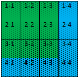
We have seen the DP algorithm that Floyd-Warshall deploys to compute APSP. Let us visualize to some extent as to how it is done for 4 vertices.

What Cells Are Used to Optimize

The computation will be done using k = 1 to 4, in the following order – starting with cell 1-1, 1-2, . . . . .2-1, 2-2, …….3-1, ……. 4-3, 4-4.

At first, using k = 1.

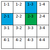
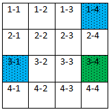
Let us see how the paths are improving using the following two examples.

dist[2][3] = min (dist[2][3],  dist[2][1] + dist[1][3])

1

and dist[3][4] = min (dist[3][4],  dist[3][1] + dist[1][4])

2

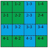
We see that for k = 1, all paths are optimized using paths from 1st (kth) row and 1st (kth) column.

Kth Row and Column do not Change

What about paths on kth row and kth column?

dist[1][2] = min(dist[1][2], dist[1][1] + dist[1][2]) – well, there is no point in updating dist[1][2] by adding something more to it.

So we see, at a certain kth iteration, kth row and kth column used to update the rest of the paths while they themselves are not changed.

At k = 1

3

At k = 2

4

At k = 3

5

At k = 4

6

Consider Only 3X3 Matrix Was Computed

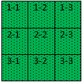
Now assume that we did not consider that we had 4 vertices. Rather we considered that we had 3 vertices and completed APSP computations for all paths in the 3X3 matrix. We ignored the 4th row and column altogether.

So we have APSP computed for the following matrix using k = 1, 2 and 3.

7

Add 4th Vertex

Let’s say, 4th vertex arrives now. First, we can compare the computations used for the above 3X3 matrix with the same for the 4X4 matrix as shown earlier and find out what all computations need to be done now to extend this 3X3 matrix to 4X4 matrix to accommodate the new 4th vertex.

We will find that at first we have to optimize the 4th row and column using k = 1, 2 and 3. Let us do that.

8

Note that at this point, 4th row and column are not used to optimize paths for the older 3X3 matrix. So now that we have the 4th row and column optimized using k = 1, 2 and 3, we have to optimize that 3X3 matrix using k = 4.

9

This way, we don’t miss out any computation had we considered all the 4 vertices at one go. And thus we are done with optimizing all the paths in the 4X4 matrix.

Code

dist[][] //APSP matrix, already computed for n-1 vertices

p[][] //predecessor matrix, already computed for n-1 vertices


dist[n][] = ∞

dist[][n] = ∞

dist[n][n] = 0


for each edge (i, n)

  dist[i][n] = weight(i, n)

  p[i][n] = n


for each edge (n, i)

  dist[n][i] = weight(n, i)

  p[n][i] = i


for k = 1 to n-1

  for i = 1 to n-1

    if dist[i][n] > dist[i][k] + dist[k][n]

      dist[i][n] = dist[i][k] + dist[k][n]

      p[i][n] = p[i][k]

  for j = 1 to n

    if dist[n][j] > dist[n][k] + dist[k][j]

      dist[n][j] = dist[n][k] + dist[k][j]

      p[n][j] = p[n][k]


for i = 1 to n-1

    for j = 1 to n-1

      if dist[i][j] > dist[i][n] + dist[n][j]

        dist[i][j] = dist[i][n] + dist[n][j]

        p[i][j] = p[i][n]

Complexity

The complexity for this incremental building for a new vertex is clearly O(n2). That makes sense. After all, for n vertices the cost is O(n3) that is the cost of Floyd-Warshall, had all n vertices were considered at one go.

But this incremental building makes a huge difference. For example, consider that we have 1000 vertices for which we have already computed APSP using 1 billion computations. Now that 1001st vertex arrives, we can accommodate the new vertex with a cost of 1 million (approx.) computations instead of doing 1 billion+ computations again from the scratch – something that can be infeasible for many applications.

Printing Arbitrage Path

We can find the first negative cycle by looking (for a negative value) at the diagonals of the dist[][] matrix, if exists and then print the associated path. For path reconstruction, we can follow the steps as described here.

GitHub: Code will be updated in a week

Index

Dijkstra’s Algorithm

10th Friday Fun Session – 17th Mar 2017

Dijkstra’s algorithm is a Single-Source Shortest Path (SSSP) algorithm developed by Edsger Wybe Dijkstra. It uses a greedy process and yet finds the optimal solution. It looks similar to Breadth-first search.

Compare to Bellman-Ford

It is asymptotically the fastest SSSP algorithm, at a cost O(|E|+|V|log|V|), when min-priority queue implemented by Fibonacci heap is used.

That is quite cheap, given Bellman-Ford’s complexity of O(|V||E|) to find the same, something that can become prohibitively expensive for a dense graph having |V|2 edges.

However, while Bellman-Ford can work with negative edge and can detect negative cycle, Dijkstra’s algorithm cannot work with negative edge. Since it cannot work with negative edge, there is no question of detecting negative cycle at all.

Standard Algorithm

dist[] //shortest path vector

p[] //predecessor vector, used to reconstruct the path

Q //vertex set

for each vertex v in Graph
  dist[v] = ∞
  p[v] = undefined
  add v to Q

dist[s] = 0

while Q is not empty
  u = vertex with min dist[] value
  remove u from Q

  for each neighbor v of u
    alt = dist[u] + weight(u, v)
    if alt < dist[v]
      dist[v] = alt
      p[v] = u

return dist[], p[]

Given source vertex s, it finds the shortest distance from s to all other vertices. At first, it initializes dist[] vector to infinite to mean that it cannot reach any other vertex. And sets dist[s] = 0 to mean that it can reach itself at a cost of 0, the cheapest. All vertices including itself are added to the vertex set Q.

Then, it chooses the vertex with min dist[] value. At first, s (set to u) would be chosen. Then using each of the outgoing edges of u to v, it tries to minimize dist[v] by checking whether v can be reached via u using edge (u, v). If yes, dist[v] is updated. Then again it retrieves vertex u with the cheapest dist[u] value and repeats the same. This continues till Q is not empty. Whenever, a vertex u is removed from Q, it means that the shortest distance from s to u is found.

Since we are retrieving |V| vertices from Q, and for each vertex, trying with all its edges (=|V|, at max), to minimize distance to other vertices, the cost can be |V|2.

So, here we see a greedy process where it is retrieving the vertex with min dist[] value.

Since retrieving a vertex u from Q means that we found the minimum distance from s to u, if we are solving shortest path from a single source s to a single destination d, then when u matches the destination d, we are done and can exit.

It can also be noted that from source s, we find the shortest distances to all other vertices, in the ascending order of their distances.

Finally, we see that dist[] vector is continuously changing. And each time when we retrieve a vertex u, we choose the one with min dist[] value. That indicates using min-priority queue might be the right choice of data structure for this algorithm.

Using Fibonacci Heap

dist[] //shortest path vector
p[] //predecessor vector, used to reconstruct the path
Q //priority queue, implemented by Fibonacci Heap

dist[s] = 0

for each vertex v
  if(s != v)
    dist[v] = ∞
    p[v] = undefined
  
  Q.insert_with_priority(v, dist[v]) // insert

while Q.is_empty() = false
  u = Q.pull_with_min_priority() // find min and delete min
  
  for each neighbor v of u
    alt = dist[u] + weight(u, v)
    if alt < dist[v]
      dist[v] = alt
      p[v] = u
      Q.decrease_priority(v, alt) //decrease key

return dist[], p[]

In the above algorithm, we have used a function called decrease_priority(), something that is absent in standard priority queue but present in Fibonacci heap. So the above algorithm is implemented using Fibonacci heap.

Fibonacci heap is a special implementation of a priority queue that supports decrease key (decrease_priority()) operation. Meaning, we can decrease the value of a key while it is still inside the priority queue. And this can be achieved by using constant amortized time for insert, find min and decrease key operation and log (n) time for delete min operation.

As for cost, since we have called delete operation for each of the v vertices, and we have treated each of the |E| edges once, the cost here is O(|E|+|V|log|V|), as mentioned at the beginning of this post, as the cost of Dijkstra’s algorithm.

Using Standard Priority Queue

Standard priority queue implementation takes log (n) time for both insert and delete operation and constant time for find min operation. But there is no way to change the key value (decrease key) while the item is still in the priority queue, something Dijkstra’s algorithm might need to do quite frequently as we have already seen.

If standard priority queue is used, one has to delete the item from the priority queue and then insert into it again, costing log (n) each time, or an alternative to that effect. However, as long as standard priority queue is used, it is going to be slower than Fibonacci heap. With standard priority queue, the algorithm would look like below:

dist[] //shortest path vector
p[] //predecessor vector, used to reconstruct the path
Q //standard priority queue

for each vertex v
  dist[v] = ∞
  p[v] = undefined

dist[u] = 0
Q.insert_with_priority(u, dist[u]) // insert

while Q.is_empty() = false
  u = Q.pull_with_min_priority() // find min and delete min
  
  for each neighbor v of u
    alt = dist[u] + weight(u, v)
    if alt < dist[v]
      dist[v] = alt
      p[v] = u
      insert_with_priority(v, alt) //insert v 
                                     even if already exists 
return dist[], p[]

There are two differences from the earlier algorithm:

First, we have not inserted all vertices into the standard priority queue at first, rather inserted the source only.

Second, instead of decreasing priority that we cannot do using standard priority queue, we have kept on inserting vertex v when dist[v] decreases. That might mean, inserting a vertex v again while it is already there inside the queue with a higher priority/dist[v]. That is another way of pushing aside the old entry (same v but with higher priority) out of consideration for the algorithm. When shortest distances from source s to all other vertices v are found, those pushed aside vertices will be pulled one by one from the priority queue and removed. They will not affect dist[] vector anymore. And thus the queue will be emptied and the algorithm will exit.

Negative Edge

Please check Dijkstra’s Problem with Negative Edge for further details.

Index

Floyd-Warshall Algorithm

35th Friday Fun Session – 29th Sep 2017

Floyd-Warshall, also known as Roy-Warshall is an All-Pairs Shortest Path (APSP) algorithm developed by Robert Floyd, Bernard Roy, and Stephen Warshall. It is an example of dynamic programming that uses 3 nested loops. At a cost O(|V|3), it is quite impressive, given that Bellman-Ford might encounter the same cost (O(|V||E|)) to find only Single Source Shortest Path (SSSP) for dense graph having |V|2 edges. Floyd-Warshall can work with negative edges just like Bellman-Ford. After all, both are based on dynamic programming. As for detecting negative cycle, once again, both can detect it. However, in presence of negative cycle, results from both are invalid.

Three Nested Loops

dist[][] //shortest path matrix
p[][] //predecessor matrix, used to reconstruct the path

dist[][] = ∞

for each vertex i
  dist[i][i] = 0

for each edge (i, j)
  dist[i][j] = weight(i, j)
  p[i][j] = j

for k = 1 to |V|
  for i = 1 to |V|
    for j = 1 to |V|
      if dist[i][j] > dist[i][k] + dist[k][j]
        dist[i][j] = dist[i][k] + dist[k][j]
        p[i][j] = p[i][k]

To compute the shortest path between any pair (s, t), we have considered each of the |V| vertices as intermediate points k, and chosen the cheaper between i) existing (s, t) and ii) the sum of s to k and then from k to t, meaning s to t via k.

Short-circuiting an SSSP?

Does it mean that we can derive a SSSP solution for any pair (s, t), at a cost of O(|V|2)? To be precise, can we do the following?

for k = 1 to |V|
  if dist[i][j] > dist[i][k] + dist[k][j]
    dist[i][j] = dist[i][k] + dist[k][j]

After all, we have relaxed via all the intermediate nodes. Well, that will not work! Why?

Dynamic Programming

If we want to get the shortest path between (i, j) using k (1 to k) intermediate nodes then we have to choose the cheaper between the below paths:

  1. Without using k: dist[i][j] using intermediate nodes 1 to k-1.
  2. Using k: dist[i][k] + dist[k][j], where both dist[i][k] and dist[j][k] should make use of intermediate nodes 1 to k-1.

At k = 0, dist[][] is initialized using edge weights where exists, 0 for diagonals (dist[v][v]) and infinite for the rests.

An Example

Suppose, we want to compute dist[2][3] when k = 5.

Then, dist[2][3] = min { dist[2][3], dist[2][5] + dist[5][3] }

Here, all three distances – dist[2][3], dist[2][5] and dist[5][3] must already use intermediate nodes 1 to 4. Meaning, dist[2][5] is not the static cost set at k=0; possibly the edge cost, 0 or infinite. Rather, dist[2][5] is already computed using k from 1 to 4. Similarly, dist[5][3] (and dist[2][3] as well) is also computed using k from 1 to 4.

In other words, we cannot compute a certain dist[s][t] alone, using the intermediate nodes 1 to k. Rather for each intermediate node k, we need to compute dist[i][j] progressively, using the 3 nested loops, as shown earlier.

Obviously we can use recursion without the loops. That will not save any work for us. In fact, while using recursion, if we are not reusing existing solutions for the sub-problems, we will repeat the computation – something very expensive.

Path Reconstruction

The predecessor matrix p, keeps track of the shortest path. If we have to find the best path from s to t, we know for sure that we start with s. We print s. To know where we went from there, we have to look at p[s][t]. If that is t, we are done as that is the destination. However, if that is not the case, that means we find another node r. Then we know from s we went to an intermediate node r. So this becomes the new start s for the rest of the path. However, destination remains the same t. Again we look at p[s][t] and continue the same till we reach t, all along printing r (=p[s][t]).

Incremental Node Addition

Suppose as of now, we have 4 nodes and APSP is computed. At this point 5th node arrives, along with some edges connecting the existing nodes. Instead of computing APSP from the scratch, at a cost of O(|V|3) = O(125), we can use the already computed APSP and extend that to complete it for 5 nodes, at a cost of O(|V|2) = O(25).

Adjusting Edge Weight Changes

What if weight for an edge changes (increases or decreases)? Do we need to re-compute APSP from scratch? Or we can adjust the existing results using some partial computations?

Index

Solution – Choosing Oranges

38th Friday Fun Session – 3rd Nov 2017

Given a set of goodness scores of oranges and a window length, we need to find the highest scoring oranges within the window as we move it from left to the end.

This is the solution for JLTI Code Jam – Oct 2017.

Using priority queue

Suppose we have n scores and the window length is m. We can simply move the window from left to to right and take (consecutive) m scores within the window and each time compute the max of them, and output it, if it is already not outputted. Finding max from m scores would take O(m) and as we do it n times (n-m+1 times, to be precise), the complexity would be O(mn). However, it was expected that the complexity would be better than this.

Alternatively, we can use a max-heap, where we push each score as we encounter it. At the same time, we retrieve the top of the max-heap and if all is fine – output it. By if all is fine, we mean to say, we need to make sure that the orange has not been already outputted and that it belongs to the current window. At the same time, if the top item is out-dated, we can pop it, meaning take it out of the heap. Note that, max-heap is a data structure that retains the max element at the top.

Let us walk through an example

Let us take the first example as mentioned here. For the scores 1 3 5 7 3 5 9 1 2 5 with window size 5, let us walk through the process.

At first, we push the first 4 items (4 is one less than the window size 5). The max-heap would look like: 1 3 5 7 where 7 is the top element.

Then for each of the remaining items, we do the following:

  1. If the (new) item is greater than or equal to the top item in the max-heap, pop it (out) and push the new item into it. Output the new item (if the same orange is not already outputted). We do it because the new item is the max in the present window. And the existing top one is of no further use. We can now move to the next item.
  2. Keep on popping the top as long it is not one belonging to the current window. We do it, as we are interested to find the max within the window, not the out-dated ones those are no longer inside the window.
  3. Output the top (if the same orange is not already outputted). We do it as it the max within the current window.
  4. If the top item is the oldest (left-most/first/earliest/starting one) in the current window, pop it. We do it because this item is going to go out of the window as the next item gets in.

Score 3:

3 is not >= 7 (top in heap)

Existing top (7) is within the current window. Output it.

Push 3; max-heap looks like: 1 3 3 5 7

Score 5:

5 is not >= 7 (top in heap)

Existing top (7) is within the current window (3 5 7 3 5). But this orange is already outputted (we can use index of the item to track it, meaning instead of just pushing the score, retain the index along with it). No output this time.

Push 5; max-heap looks like: 1 3 3 5 5 7

Score 9:

9 >= 7 (top in heap)

Pop 7, push 9, output 9.

New max-heap: 1 3 3 5 5 9

Score 1:

1 is not >= 9 (top in heap)

Existing top (9) is within the current window. But this orange is already outputted. No output this time.

Push 1; max-heap looks like: 1 1 3 3 5 5 9

Score 2:

2 is not >= 9 (top in heap)

Existing top (9) is within the current window. But this orange is already outputted. No output this time.

Push 2; max-heap looks like: 1 1 2 3 3 5 5 9

Score 5:

Existing top (9) is within the current window. But this orange is already outputted. No output this time.

Push 5; max-heap looks like: 1 1 2 3 3 5 5 5 9

No item left. We are done!

Finally, output is 7, 9.

Complexity

If we closely observe, we see that the size of the max-heap would be always around m. Because, if the new item is greater or equal we are popping the top – hence the max-heap size is not increasing. If new item is smaller, we are pushing it and the size of the max-heap is increasing – true; but then soon the top would be out-dated and then we would pop that. So the max-heap size remains around m. Pushing (in) or popping (out) an item would cost log m, and since we would do it n times – the complexity would be O(n log m). Please note that getting the top of the max-heap costs O(1).

GitHub: Choosing Oranges

Index

Graced by Your Presence


Friday Fun Session Participants

Those of us who participate(d) our weekly learning and discussion session:

  1. Bala Krishnan
  2. Tang Biao
  3. Vignesh Shankar
  4. Chia Wei Woo
  5. Mahadevan Hariharan
  6. Ramakrishnan Kalyanaraman
  7. William Lim
  8. Srila Das Bhattacharya
  9. Sravani Vanukuru
  10. Kristipi Valledor
  11. Jeffrey Quiatchon
  12. Jothi Kiruthika
  13. Sayed Neda Fatima
  14. Sreenivasulu Gotla
  15. Vishal Gupta
  16. French Jean Palma Jumawan
  17. Gopi Krishna Pasupuleti
  18. Htet Aung Nay
  19. Aquib Javed Momin
  20. Pravinkarthy Ravi
  21. Rishabh Mangal
  22. Sunil Koli
  23. Vikas Pai
  24. Sandip Dangat
  25. Hui Ling Chong
  26. Srinivasa Puchakayala Reddy
  27. Manikandan Chandran
  28. Sharon Wong
  29. Uma Maheswary Ganesan
  30. Ishwarya Sridharan
  31. Aristotle Tiru
  32. Balamurugan Chennarayaperumal
  33. Aarti Piskala Dhanabalan
  34. Karthik Kumar
  35. Sunil Khamkar
  36. Handy Toh Torres
  37. Daniel Vo
  38. Srinivasan Badri Prasad
  39. Parthasarathi Murugaiyan
  40. Hieu Nguyen Van
  41. Manikandan Panneerselvam
  42. Jayamaran Ayilu
  43. Muukta Kedar
  44. Gaurav Singh
  45. Vikas Kitawat
  46. Tanveer Shaikh
  47. Vishal Jain
  48. Dipti Saurabh Shindhe
  49. Samir Tank
  50. Bhushan Patil
  51. Munendra Tomar
  52. Prabakaran Boopathi
  53. Vikraman Sridharan
  54. Srikanth Rokkam
  55. Santhosh Kumar Janakiraman
  56. Christabel Merline
  57. Ankit Jain
  58. Neethila Arasi
  59. Hari Gopal Raman
  60. Sheryl Teo
  61. Jocelyn Pacson Maranan
  62. Kannan Palanisamy
  63. Chitra Muthu
  64. Chaitanya Joshi
  65. Billie Santiago
  66. Thandar Win
  67. Julius Pedroso
  68. Chinta Nagendra Babu
  69. Lourdu Michael Sam
  70. Gayan Gunarathne
  71. Amit Gupta
  72. Akshatha Davasam
  73. Parimi Chowdary
  74. Haribabu Gattipati
  75. Rajesh Mutyala
  76. Janani Vijayan
  77. Prashasti Shandilya
  78. Anju Singh
  79. Akash Mule
  80. Anclyn Demol Yballe
  81. Gopal Chandra Das

Problems in JLTi Code Jam

JLTi Code Jam Problems

Year 2018

Mar (13th) – Currency Arbitrage with Increasing Rate

Feb (12th) – Currency Arbitrage with Decreasing Rate

Jan (11th) – Currency Arbitrage

Year 2017

Dec (10th) – Sprint Completion Time

Nov (9th) – RC Election Result

Oct (8th) – Choosing Oranges

Sep (7th) – Team Lunch

Aug (6th) – FaaS

Jul (5th) – Scoring Weight Loss

Jun (4th) – Manipulating Money Exchange

May (3rd) – Making Money at Stock Exchange

Apr (2nd) – Company Tour to Noland

Mar (1st) – No Two Team Member Next to Each Other

Index

Other Posts

Topics in Friday Fun Session

Friday Fun Session Topics

Year 2019

Jul

4th Jul 2019 (110th) – Detecting the Start Node of a Loop in a Singly Linked List, if Exists

Jun

27th Jun 2019 (109th) – Building the Highest Stack of Cuboids of Varrying Length, Height, and Width Without Rotating in Non-Increasing Order From Bottom to Top

20th Jun 2019 (108th) – Detecting Poison in 1 Out of 2n bottles Using n Strips That Changes Color Only When Poison is Poured On it

13th Jun 2019 (107th) – Searching in a Sorted and Rotated Array

6th Jun 2019 (106th) – Delete a Node from BST

May

30th May 2019 (105th) – Retrieving a Random Item from BST

23rd May 2019 (104th) – Optimizing SQL Queries Using Join Hints

16th May 2019 (103rd) – Largest Rectangular Area in a Histogram at O(n)

9th May 2019 (102nd) – Efficient Construction of Hierarchical Dropdown for UI

2nd May 2019 (101st) – Hierarchical and Recursive Queries in T-SQL

Apr

25th Apr 2019 (100th) – Segment Tree (Query and Update)

18th Apr 2019 (99th) – Segment Tree (Building)

11th Apr 2019 (98th) – Maximum Rectangular Area in Histogram (Divide and Conquer)

4th Apr 2019 (97th) – Trapping Rain Water

Mar

28th Mar 2019 (96th) – Dutch National Flag Problem

21st Mar 2019 (95th) – Permutation

14th Mar 2019 (94th) – Post-order sequence to binary tree, check if BST

7th Mar 2019 (93rd) – Pre-order sequence to binary tree, check if BST

Feb

28th Feb 2019 (92nd) – Task Dependencies, Build Execution Order, if Any (using DFS)

21st Feb 2019 – Missed, On Leave

14th Feb 2019 (91st) – Build BST in an Efficient Way to Count Height of Each Node (Contd.)

7th Feb 2019 (90th) – Build BST in an Efficient Way to Count Height of Each Node (Contd.)

Jan

31st Jan 2019 (89th) – Build BST in an Efficient Way to Count Height of Each Node (Contd.)

25th Jan 2019 (88th) – Build BST in an Efficient Way to Count Height of Each Node

17th Jan 2019 (87th) – Common First Ancestor of Two Nodes in a Binary Tree with All Unique Values

10th Jan 2019 (86th) – Check if a Binary Tree is Balanced

3rd Jan 2019 (85th) – Number of Paths with a Certain Sum in a Binary Tree (Top-down)

Year 2018

Dec

27th Dec 2018 (84th) – Number of Subsequences Making a Certain Sum In an Array

20th Dec 2018 (83rd) – Number of Paths with a Certain Sum in a Binary Tree (Bottom-up)

13th Dec 2018 (82nd) – Binary Tree to Doubly Linked List

5th Dec 2018 (81st) – Given a BST, Find All Input Sets That Can Build it

Nov

28th Nov 2018 (80th) – Number of ways a BST can be built with n distinct keys

21st Nov 2018 (79th) – Merge Two Lists in All Possible Ways Preserving Relative Order of Elements Within Each List

14th Nov 2018 (78th) – Two-way/Bidirectional Search BFS

7th Nov 2018 (77th) – Detecting Cycle in a Directed Graph

Oct

31st Oct 2018 (76th) – Drawing with HTML5 <canvas> and JavaScript, Rotation of Axes, Arrow Drawing

24th Oct 2018 (75th) – CA, ICA, Chain of Trust

17th Oct 2018 (74th) – How does SSL/TLS work

10th Oct 2018 (73rd) – Self-signed SAN Certificate for localhost Using OpenSSL

3rd Oct 2018 (72nd) – Gradient Descent

Sep

26th Sep 2018 (71th) – Simple Linear Regression Using Gradient Descent

19th Sep 2018 (70th) – Simple Linear Regression Using Linear Least Squares

12th Sep 2018 (69th) – Multiple Linear Regression Demo Using R

5th Sep 2018 (68th) – Cycle Detection Using Union by Rank and Path Compression in an Undirected Graph

Aug

29th Aug 2018 (67th) – Union by Rank and Path Compression

22nd Aug 2018 – Missed, Public Holiday

15th Aug 2018 (66th) – Stable Roommates Problem (continued)

8st Aug 2018 (65th) – Stable Roommates Problem (continued)

1st Aug 2018 (64th) – Stable Roommates Problem

Jul

25th Jul 2018 (63rd) – 2-d Array Printing in Spiral order

18th Jul 2018 (62nd) – Stable Marriage Problem (continued)

11th Jul 2018 (61st) – Stable Marriage Problem

4th Jul 2018 (60th) – DFS

Jun

27th Jun 2018 (59th) – BFS

20th Jun 2018 – Cancelled

13th Jun 2018 (58th) – Ford-Fulkerson Method (Max-flow)

6th Jun 2018 – Missed, On Leave

May

30th May 2018 – Missed, On Leave

23rd May 2018 (57th) – Karger’s Algorithm (Minimum cut)

16th May 2018 (56th) – Solution – Currency Arbitrage with Increasing Rate

11th May 2018 – Cancelled

4th May 2018 – Cancelled

Apr

27th Apr 2018 – Cancelled

20th Apr 2018 – Cancelled

13rd Apr 2018 – Cancelled

6th Apr 2018 – Cancelled

Mar

30th Mar 2018 – Missed, Public Holiday

23rd Mar 2018 (55th) – Bitcoin – Simple Payment Verification (SPV)

16th Mar 2018 (54th) – Cryptographic Hash Function – Properties

9th Mar 2018 (53rd) – Collation in MS SQL Server

2nd Mar 2018 (52nd) – Solution – Currency Arbitrage with Decreasing Rate

Feb

23rd Feb 2018 (51st) – Merkle Tree

16th Feb 2018 – Missed, Chinese New Year

9th Feb 2018 (50th) – RSA

2nd Feb 2018 (49th) – Solution – Currency Arbitrage

 Jan

26th Jan 2018 (48th) – Overview of Bitcoin and Blockchain

19th Jan 2018 (47th) – Johnson’s Algorithm

12th Jan 2018 (46th) – Dijkstra’s Problem with Negative Edge

5th Jan 2018 (45th) – Solution – Sprint Completion Time

Year 2017

Dec

29th Dec 2017 – Missed, On Leave

22nd Dec 2017 – Missed, On Leave

15th Dec 2017 (44th) – Rod Cutting Problem

8th Dec 2017 (43rd) – Task Scheduling – Unlimited Server

1st Dec 2017 (42nd) – Solution – RC Election Result

Nov

24th Nov 2017 (41st) – Traveling Salesman Problem (Brute force and Bellman–Held–Karp)

17th Nov 2017 (40th) – Hamiltonian Path

10th Nov 2017 (39th) – Coin Exchange – Min Number of Coins

3rd Nov 2017 (38th) – Solution – Choosing Oranges

Oct

27th Oct 2017 – Missed, On Leave

20th Oct 2017 (37th) – Coin Exchange – Number of Ways

13th Oct 2017 – Missed, JLT D&D

6th Oct 2017 (36th) – Solution – Team Lunch

Sep

29th Sep 2017 (35th) – Floyd-Warshall Algorithm

22nd Sep 2017 (34th) – Executing SP Using EF; Transaction in Nested SP

15th Sep 2017 (33rd) – Solution – FaaS; Pseudo-polynomial Complexity

8th Sep 2017 – Missed, JLT Family Day

1st Sep 2017 – Missed, Hari Raya

Aug

25th Aug 2017 (32nd) – Multithreaded Programming

18th Aug 2017 (31st) – Knapsack Problem

11th Aug 2017 (30th) – Vertex Coloring

4th Aug 2017 (29th) – Solution – Scoring Weight Loss

Jul

28th Jul 2017 (28th) – Minimum Spanning Tree – Kruskal and Prim

21st Jul 2017 (27th) – Pseudorandom Number Generator

14th Jul 2017 (26th) – Rete Algorithm

7th Jul 2017 (25th) –  Solution – Manipulating Money Exchange

Jun

30th Jun 2017 (24th) –  Rules Engine

23rd Jun 2017 (23rd) –  Inducting Classification Tree

16th Jun 2017 (22nd) –  Incision into Isolation Level; Interpreting IIS Internals; Synchronizing Web System

9th Jun 2017 (21st) –  Maximum Subarray Problem

2nd Jun 2017 (20th) –  Solution – Making Money at Stock Market

May

26th May 2017 (19th) –  Understanding Correlation Coefficient; k-NN Using R

19th May 2017 (18th) –  k-d Tree and Nearest Neighbour Search

12th May 2017 (17th) –  Bellman Ford Algorithm

5th May 2017 (16th) –  Solution – Company Tour 2017 to Noland

Apr

28th Apr 2017 (15th) –  Models in Machine Learning; k-Nearest Neighbors (k-NN)

21st Apr 2017 (14th) – Edit/Levenshtein Distance

14th Apr 2017 – Missed, Good Friday

7th Apr 2017 (13th) – Solution – No Two Team Member Next to Each Other

Mar

31st Mar 2017 (12th) – N-queens

24th Mar 2017 (11th) – Longest Common Subsequence (LCS)

17th Mar 2017 (10th) – Dijkstra’s Algorithm

10th Mar 2017 (9th) – Infix, Prefix (Polish), Postfix (Reverse Polish)

3rd Mar 2017 (8th) – Order 2-D Array in all Directions & Find all Triplets with Sum Zero in an Array

Feb

24th Feb 2017 (7th) – Trailing Zeros in a Factorial

17th Feb 2017 (6th) – Is this Tree a BST?

10th Feb 2017 (5th) – Given a Number, Find the Smallest Next Palindrome

3rd Feb 2017 (4th) – Merge n Sorted Lists, Each Having m Numbers, Into a Sorted List

Jan

27th Jan 2017 – Missed, Chinese New Year Eve

20th Jan 2017 (3rd) – Shortest Exit from Maze

13rd Jan 2017 (2nd) – Finding Fibonacci – Exponential vs. Linear

6th Jan 2017 (1st) – Gmail API with OAuth 2.0

Other Posts

Problems in JLTi Code Jam