Johnson’s Algorithm

47th Friday Fun Session – 19th Jan 2018

We have seen why Dijkstra’s algorithm cannot work with negative edge and that we cannot trivially add a constant to each of the edge weights and make them non-negative to proceed further. It is where Johnson’s algorithm comes into play. It finds a special set of offset values to remove the negative edges (change the negative edge weights to non-negative edge weights) and now this transformed graph is all set to work with Dijkstra’s algorithm.

How Does Johnson’s Algorithm work?

Johnson’s algorithm starts with a graph having negative edge(s). Let’s go through it using an example as shown below.

1

Add a New Node

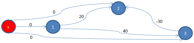
It then adds a new vertex, let’s call it s, with edges starting from it and ending to each of the vertices of the existing graph, each having a cost of 0, as we have done earlier.

2.png

Apply Bellman-Ford

Then it applies Bellman-Ford, a Single Source Shortest Path (SSSP) algorithm that can work with a graph having negative edge(s). We will use s as the source, and find shortest path from it to all other vertices.

We also need to check whether a negative cycle exists, something that Bellman-Ford can detect. If it exists then we cannot proceed further as we cannot find shortest path in a graph with negative cycle. In our example graph, there is no negative cycle.

We find d[s, 1] = 0, d[s, 2] = -30, and d[s, 3] = 0 as shown below, using this code where d[s, t] indicates the shortest path from s to t.

3.png

Adjust Original Edge Weights

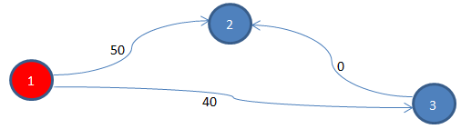
Now using these shortest path costs, original edges will be updated using the formula: w’[u, v] = w[u, v] + d[s, u] – d[s, v]. Applying the same for the original 3 edges in the original graph, we find,

w’[1, 2] = w[1, 2] + d[s, 1] – d[s, 2] = 20 + 0 – (-30) = 50

w’[1, 3] = w[1, 3] + d[s, 1] – d[s, 3] = 40 + 0 – 0 = 40

w’[3, 2] = w[3, 2] + d[s, 3] – d[s, 2] = (-30) + 0 – (-30) = 0

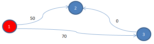
Now that we have adjusted the original edge costs, the new (cost) adjusted graph (without s and associated edges) does not have any more negative edge. Let’s see how the cost adjusted graph looks like.

4

Apply Dijkstra

With this non-negative edge graph we can proceed with Dijkstra’s algorithm. For each shortest path found in this graph from u to v, we have to adjust back the cost by subtracting d[s, u] – d[s, v] from it.

Is the Shortest Path Still the Same?

We are adjusting edge cost to remove negative edge. That way, we are changing the graph to some extent. However, while doing so we must preserve certain things of it. What was the cheapest cost in the original graph must still remain the cheapest path in the transformed graph. Let’s first verify whether that is indeed the case.

We will first look at the original graph (before edge cost adjustment). Let’s take a certain source destination pair (1, 2). There are two paths to reach from vertex 1 to vertex 2.

The first one (original):

d1[1, 2]

= from vertex 1 to vertex 2 directly using edge 1->2

= 20.

The second one (original):

d2[1, 2]

= from vertex 1 to 3 and then from 3 to 2

= 40 + (-30)

= 10.

Now let’s see how the costs of the same two paths change in the new cost adjusted graph.

The first one (cost adjusted):

d’1[1, 2]

= from vertex 1 to vertex 2 directly using edge 1->2

= 50.

The second one (cost adjusted):

d’2[1, 2]

= from vertex 1 to 3 and then from 3 to 2

= 40 + 0

= 40.

We see both the path costs have increased by 30, a constant. So what was earlier the shortest from vertex 1 to vertex 2, in the original graph, which was the second path, using two edges: edge 1->3 and edge 3->2, still remains the shortest path in the cost adjusted graph.

So how did that happen? Let’s have a closer look as to how the path cost changes.

The first one (cost adjusted):

d’1[1, 2]

= w’[1, 2]

= w[1, 2] + d[s, 1] – d[s, 2]

= d1[1, 2]  + d[s, 1] – d[s, 2]

The second one (cost adjusted):

d’2[1, 2]

= w’[1, 3] + w’[3, 2]

= w[1, 3] + d[s, 1] – d[s, 3] + w[3, 2] + d[s, 3] – d[s, 2]

= w[1, 3] + d[s, 1] + w[3, 2] – d[s, 2]

= w[1, 3] + w[3, 2] + d[s, 1] – d[s, 2]

= d2[1, 2] + d[s, 1] – d[s, 2]

So we see both the paths, with a certain source u and a certain destination v, have increased with a constant cost = d[s, u] – d[s, v], where s is the extra node that we added before applying Bellman-Ford algorithm.

We can easily find, no matter how many paths are present between a certain source s and a certain destination v, and no matter how many edges each of those paths uses, each of them would be adjusted by adding a constant cost = d[s, u] – d[s, v] to it. And hence, the shortest path in the original graph remains the shortest path in the new cost adjusted, non-negative edge graph.

Let’s consider a path that goes through 5 vertices: u, x1, x2, x3, and v.

In the cost adjusted graph the cost

d’[u, v]

= w’[u, x1] + w’[x1, x2] + w’[x2, x3] + w’[x3, v]

= w[u, x1] + d[s, u] – d[s, x1] + w[x1, x2] + d[s, x1] – d[s, x2] + w[x2, x3] + d[s, x2] – d[s, x3] + w[x3, v] + d[s, x3] – d[s, v]

= w[u, x1] + d[s, u] + w[x1, x2] + w[x2, x3] + w[x3, v] – d[s, v]

= w[u, x1] + w[x1, x2] + w[x2, x3] + w[x3, v] + d[s, u] – d[s, v]

= d[u, v] + d[s, u] – d[s, v]

By generalizing the above, we see that a constant cost d[s, u] – d[s, v] is getting added to all paths from u to v.

Are all Negative Edge Removed?

The second thing that we need to prove is: no longer there exists a negative edge in the adjusted graph. After applying Bellman-Ford, we computed the shortest paths from source s. Let’s assume, d[s, u] and d[s, v] are the shortest paths from s to any two vertices, u and v, respectively. In that case, we can say,

d[s, v] <= d[s, u] + w[u, v]

=> 0 <= d[s, u] + w[u, v] – d[s, v]

=> 0 <= w[u, v] + d[s, u] – d[s, v]

=> 0 <= w’[u, v]

We prove that the new edge cost, w’[u, v] is always non-negative.

Why Would We Use Johnson’s algorithm?

So here with Johnson’s algorithm, first we use Bellman-Ford to get a set of values; using which we transform the graph with negative edge to a graph with all non-negative edges so that we can apply Dijkstra’s algorithm.

But why would anyone want to do that? After all, both Bellman-Ford and Dijkstra are SSSP algorithms. What is the point of using one SSSP algorithm to transform a graph so that another SSSP algorithm can be used on the transformed graph?

Dijkstra’s Algorithm is Faster

Well, the reason being, the latter SSSP algorithm, namely Dijkstra’s, is much faster than Bellman-Ford. So, if we need to find shortest paths many times, then it is better that first we apply a bit more expensive SSSP alogorithm – Bellman-Ford to get the graph ready to work with Dijkstra’s algorithm. Then we execute much cheaper Dijkstra’s algorithm on this transformed graph, as many times as we want – later.

Sparse Graph

But in such a situation is it not better to run an ALL-Pairs Shortest Paths (APSP) algorithm like Floyd-Warshall? After all, Floyd-Warshall can compute APSP at a cost of O(V3) while Bellman-Ford costs O(|V| * |E|) that can shoot up to O(V3), when E=|V|2 for a dense graph.

Yes, that is correct. For a dense graph Johnson’s algorithm won’t possibly be useful. Johnson’s algorithm is preferable for a sparse graph when Bellman-Ford is reasonably efficient to work with it.

Index

Currency Arbitrage with Increasing Rate

13th JLTi Code Jam – Mar 2018

After adding new node to Floyd-Warshall algorithm incrementally and dealing with decreasing rate (of an existing currency pair), the next logical thing is how to deal with increasing rate (of an existing currency pair). By an existing currency pair we mean both the currencies were already present and there was already a rate between the two.

Just like before, given that we have an existing best path cost matrix, when a rate between two currencies increases what shall we do? Once again, we have two options:  i) re-compute the cost matrix from the scratch, using Floyd-Warshall, at a cost O(V3) and ii) update the already computed cost matrix using some partial computations. This problem expects a solution using the second option.

Input:

1 USD = 1.380 SGD

1 SGD = 3.080 MYR

1 MYR = 15.120 INR

1 INR = 0.012 GBP

1 GBP = 1.29 USD

I CAD = 0.57 GBP

1 GBP = 1.30 USD

Explanation: We have 7 inputs here. Each time an input is given, we need to present an output and hence, we have 7 lines of output.

The first 6 inputs do not result in any arbitrage; we output “No luck here”.

At 7th input, we see the existing rate from GBP to USD, which was 1.29 last time, has changed (increased) to 1.30 now. With this new rate in effect, an arbitrage comes into picture now. We need to output the path that creates that arbitrage.

Since in this problem, we are dealing with only increasing rate, in input, between two currencies, rate will only increase. For example, an input like 1 GBP = 1.25 USD will never appear.

When multiple arbitrages exist, printing any one will do.

Output:

No luck here

No luck here

No luck here

No luck here

No luck here

No luck here

USD -> SGD -> MYR -> INR -> GBP -> USD

Task: For each line of input, for each new vertex, incrementally adjust/add shortest paths at a cost (time) of O(|V|2), detect the presence of an arbitrage and output as specified. Use existing solution for this.

If input contains a rate that has increased since last time, accommodate that change in the best path cost matrix using some partial computations, instead of computing the whole matrix from the scratch.

Index

Collation in MS SQL Server

53rd Friday Fun Session – 9th Mar 2018

What Does Collation Do in SQL Server?

Collation in SQL server does two things:

  1. Storage: specifies the character set/code page used to store non-Unicode data
  2. Compare and sort: determines how to compare and sort all textual data

No Bearing on Code Page of Unicode Data

Code page as specified in a collation is applicable only for non-Unicode characters. Unicode data is stored using UCS-2/UTF-16 character set (UCS-2 is a predecessor of UTF-16), code page 0, irrespective of what collation is in use. So collation has no bearing on the storage of nvarchar, nchar etc. type (Unicode) data.

Many Code Pages

Apart from code page 0 that is used for Unicode data, there are 16 other code pages for storing non-Unicode data.

SELECT
name,
COLLATIONPROPERTY(name, 'CodePage') AS [Code Page],
description
FROM ::fn_helpcollations()

Each of the around 3885 collations, as I can see in SQL Server 2012, uses one of these 17 code pages. As said, even when a collation uses one of those 16 non-Unicode code pages, for Unicode data (nvarchar etc.), code page 0 will always be used. Code page for Unicode data is not configurable. However, around 510 collations use code page 0. For them, even for non-Unicode data like varchar, code page 0 will be used.

Two Parts of a Collation Name

A collation name looks like SQL_Latin1_General_CP1_CI_AS. The first part indicates the (language and) code page. The later part CI, AS etc. indicates compare/sort rules.

No Bearing on Compare/Sort for Non-textual Data

Collation affects only textual data as far as comparing/sorting is concerned. Non-textual data like integer, date, bool, decimal etc. are not affected.

Options Associated with Collation

All the options as listed below dictate sorting preferences.

  1. Case-sensitive (_CS) – ABC equals abc or not.
  2. Accent-sensitive (_AS) – ‘a’ equals ‘ấ’ or not.
  3. Kana-sensitive (_KS) – Japanese kana characters (Hiragana and Katakana) sensitivity
  4. Width-sensitive (_WS) – full-width and half-width characters sensitivity
  5. Variation-selector-sensitive (_VSS) – related to variation selector of Japanese collations.

Collation Sets

There are many collations that can be used in SQL Server. They are broadly divided into three categories:

  1. SQL collations
  2. Windows collations
  3. Binary collations

SQL Collations

SQL collations use different algorithms for comparing Unicode and non-Unicode data. Let’s us understand using an example.

Suppose SqlDb database, as used for the below example, using SQL_Latin1_General_CP1_CI_AS (CP1 stands for code page). NameU column uses nvarchar (Unicode) while NameNU column uses varchar. Sorting on them produce two different sets of results as shown below.

SELECT
[Id],
[NameU],
[NameNU]
FROM [SqlDb].[dbo].[Test1]
ORDER BY [NameU]

1

ab comes before a-c when sorting is done based on the Unicode column.

SELECT
[Id],
[NameU],
[NameNU]
FROM [SqlDb].[dbo].[Test1]
ORDER BY [NameNU]

2.png

On the other hand a-c comes before ab when sorting is done based on the non-Unicode column.

Windows Collations

Windows collation, introduced in SQL Server 2008, uses the same algorithm for comparing both Unicode and non-Unicode data.

SqlDbU database as used below is using Windows collation Latin1_General_CI_AS. Using the same table definition and same queries as earlier, we see that both result sets are the same unlike earlier.

SELECT
[Id],
[NameU],
[NameNU]
FROM [SqlDbU].[dbo].[Test1]
ORDER BY [NameNU]

3

ab comes before a-c when sorting is done based on the Unicode column. So we see sorting results on Unicode data remain the same in both SQL and Windows collation.

SELECT
[Id],
[NameU],
[NameNU]
FROM [SqlDbU].[dbo].[Test1]
ORDER BY [NameU]

4

Once again, ab comes before a-c when sorting is done based on the non-Unicode column.

Consistent Sorting Behavior across Database and Application

One more good thing about Windows collation is that, if it is used then sorting behavior is consistent with other applications running in a computer using the same local settings.

After all, “Windows collations are collations defined for SQL Server to support the Windows system locales available for the operating system on which SQL Server instances are installed.”

For new SQL Server installation Windows collation is recommended.

Difference at a Glance

Difference between a SQL collation and its equivalent Windows collation can also be seen from the description column of the below query result.

SELECT
name,
COLLATIONPROPERTY(name, 'CodePage') AS [Code Page],
description
FROM ::fn_helpcollations()
WHERE name IN ('Latin1_General_CI_AS', 'SQL_Latin1_General_CP1_CI_AS')

5.png

As we see, (inside SQL Server) the only difference being how the sort/compare would happen for non-Unicode data.

Comparing/Sorting Unicode

Comparing/sorting results for Unicode data remain the same in equivalent (language and option being the same) SQL and Windows collation. But they will vary when options are different. In the below example, Both NameU1 and NameU2 columns are using nvarchar (Unicode) data type. But they are using two different collations having different options – the first is using a case-sensitive collation while the latter is using a case-insensitive one. Output will be based on collation option and hence they will differ.

SELECT
[Id],
[NameU1] -- uses SQL_Latin1_General_CP1_CS_AS,
[NameU2] -- uses SQL_Latin1_General_CP1_CI_AS
FROM [AbcSU].[dbo].[Test1]
ORDER BY [NameU2]

If we ORDER BY column NameU1 that is using a case-sensitive collation, we see the below result.

6

If we ORDER BY column NameU2 that is using a case-insensitive collation, we see the below result (following the same order as the data inserted into the table).

7.png

How to Set Collations

Collations can be set at server, database, and column level. Apart from that, it can be used in an expression to resolve two different collations.

Server Collation

There is a server level collation. Once set during installation, changing it would require dropping all user databases first (after generating database creation script, export data etc.), rebuilding master database etc., recreate the user database and import the data back.

Database Collation

By default, when a user database is created, it inherits server’s collation. However, it can specify its own collation as well. That way, each database can have its own collation. Database collation is the default for all string columns, temporary objects, variable names and other strings in the database. We cannot change the collation for system databases.

Once a database is created, collation for it can be further changed. However, we need to take care as to how the possible code page change would affect the existing data. Also, how the option changes, if any, would produce different query/join result.

Column Level Collation

Down the line, collation can be specified at column level (of a table). Same concerns, as to how the existing data would behave, have to be addressed.

Expression Level Collation

Collation can be specified at expression level as well – for example, to join two columns belonging to two different collations that SQL Server would otherwise complain.

Changing Collation Changes Meaning of Underlying Data

If collation is changed for a column/database, underlying code page might also change. If it differs, the new collation might render an existing char as something different in the new collation. For example, a character represented by code 100 remains the same at storage – still 100, with changing collation, but the mapped char in the new collation might be different.

For Unicode data, output/mapping remains the same. After all, there is just one code base for them.

As far as compare/sort is concerned, some of the things might change. For example, result of a query that uses a sort on a textual column may change if one of the collation options, say case-sensitivity changes. The same might affect the cardinality of a sort result. A sort result that was earlier producing a certain number of rows can produce more or less rows now.

Safe Collation Change

However, as far as changing a SQL collation to a Windows collation (or vice versa) is concerned, as long both the collation options remain the same and if the database is using only Unicode data (nvarchar etc.), it is quite safe. The below query can be used to find what all data types are used in the database table (and view) columns.

SELECT *--distinct(DATA_TYPE)
FROM INFORMATION_SCHEMA.COLUMNS
WHERE DATA_TYPE = 'varchar'

Temp Table Issues

One particularly common problem that arises from the difference in collation is to deal with temp tables. When collation of a database varies from its server’s collation, the temporary tables it creates use a different collation (server’s collation) from it. After all, temp tables are created in tempdb database and this system database follows the server’s collation. Temp table with a different collation than the database that created it works fine on its own. However, if say a join (on textual column) is required between that temp table and a table in the user database, and that is often the case, then SQL Server would complain as the collations of the two columns are different.

To avoid this issue, when temp table is defined, it is safe to specify the right (same as the database creating it with which it would do a join later) collation, for its textual columns.

Address nvarchar(10) COLLATE Latin1_General_CI_AS NULL;

Alternatively, while joining two columns belonging to different collation, we can specify what collation should be used (collation in expression).

Suppose, #T1 is using Windows collation Latin1_General_CI_AS while T2 is using SQL collation SQL_Latin1_General_CI_AS. If we want the join to take place using SQL collation then we will use the below query.

SELECT *
FROM T1
INNER JOIN T2 ON #T1.field COLLATE SQL_Latin1_General_CI_AS = T2.field

Index

Dijkstra’s Problem with Negative Edge

46th Friday Fun Session – 12th Jan 2018

Dijkstra’s algorithm cannot work with negative edge. Also, we cannot trivially add a constant to each of the edge weights and make them non-negative to proceed further.

Why Does Dijkstra’s Algorithm not Work with Negative Edge?

negative edge

In the above figure, we are trying to get shortest paths from source node 1 to all other nodes (node 2 and node 3). Since Dijkstra’s algorithm works by employing a greedy process, it outputs 20 as the shortest path cost to node 2.

As we can see, from node 1, we can go to two nodes – node 2 and node 3, at a cost of 20 and 40 respectively. Hence, going to node 2 is cheaper. And that is why, it outputs 20 to be the cheapest cost to reach node 2.

However, we know that the cheapest cost to reach node 2 is through node 3. And the associated cost is: 40 + (-30) = 10. So Dijkstra’s algorithm gets it wrong. It gets it wrong because it cannot foresee that later, a negative edge can bring down the total cost to below 20.

If we carefully observe, we see that the wrong calculation by Dijkstra’s algorithm happens due to the negative edge. Had cost from node 3 to node 2 not been negative, it could never bring down the total cost to lower than 20, after getting added to 40.

Why Does Adding a Constant Cost to Each Edge not Work?

Now that we realize, Dijkstra’s algorithm fails due to the negative edge from node 3 to node 2, having the value -30, we might be tempted to add 30 to each of the edges. We might think, this way we can remove the negative edge. And doing so would be fair; after all, we are adding the same value to each of the edges. Let’s do it and see what happens.

adjusting negative edge.png

After updating the edge costs, the graph looks as shown above. So what is the cheapest path from node 1 to node 3 now?

Well, now the cheapest cost is 50, which uses the direct edge from node 1 to node 2. But this is not supposed to be the cheapest path, right? The cheapest path was node 1 -> node 3 -> node 2, before we adjusted the edge cost. Adjusting edge cost should not change the graph. It must not change the cheapest path, right?

So why does that happen? Well, if we observe, we find that path node 1 -> node 3 -> node 2 uses two edges/segments – node 1 to node 3 and node 3 to node 2. On the other hand, path node 1 -> node 2 uses just one edge/segment. The way we have updated the edge cost – adding a constant to each path segment – is not fair to a path using more path segments. For the path that uses two path segments, which was originally the cheapest path, we have added the constant 30 twice. On the other hand, for the path that uses just one path segment, we have added 30 only once. That way, we are unfair to the path using more path segments.

We must add a constant to each of the paths, not to each of the path segments.

Solution

Johnson’s algorithm does this – add a constant cost to each path with a certain source s to a certain target t. It does so, by finding a special set of offset values to remove the negative edges from a graph. Once that is done Dijkstra’s algorithm can work. But that works in absence of a negative cycle in the graph.

Index

Other Posts

Posts, not listed in Friday Fun Session and JLTi Code Jam

  1. Dissecting Dates in the Context of C# MVC and Kendo Grid
  2. MS SQL Server Data (Table) Storage
  3. MS SQL Server Nvarchar Issues
  4. MS SQL Server Recovery Model
  5. Heartbleed Bug
  6. Cashier’s Order from DBS Online Banking
  7. FILESTREAM – Considerations, Restrictions and Limitations
  8. FILESTREAM – Setup
  9. FILESTREAM – Hardware/OS Consideration
  10. FILESTREAM – What and When
  11. Optimizing Inserts
  12. Replacing Subqueries With Join Might Drastically Boost Query Performance
  13. Are You Blindly Trusting Plans Generated by MS SQL Server?
  14. Searching Just One Record Taking Several Seconds?

Index

Problems in JLTi Code Jam

Currency Arbitrage with Decreasing Rate

12th JLTi Code Jam – Feb 2018

Here we extend the Currency Arbitrage problem that expected us to re-compute the best path cost matrix when a new currency arrived along with some rates from and/or to the existing currencies. We came up with a solution at O(n2) cost.

If we look at the currency exchange issues, we realize that new currencies are not arriving every day. Rather, rates among the existing currencies are the ones which are changing every now and then. So it’s equally, if not more, important to find a solution as to how to address the rate changes and compute the cost matrix.

Rate between two currencies can either increase or decrease. Here we will focus only on rate decrease.

Given that we have an existing best path cost matrix, when a rate between two currencies decreases what shall we do? Well, just like Currency Arbitrage problem, we have two options:  i) re-compute the cost matrix from the scratch, using Floyd-Warshall, at a cost O(V3) and ii) update the already computed cost matrix using some partial computations. This problem expects a solution using the second option.

Input:

1 USD = 1.380 SGD

1 SGD = 3.080 MYR

1 MYR = 15.120 INR

1 INR = 0.012 GBP

1 GBP = 1.30 USD

I CAD = 0.57 GBP

1 GBP = 1.29 USD

Explanation: We have 7 inputs here. Each time an input is given, we need to present an output and hence, we have 7 lines of output. We already know how to incrementally add a new currency. The first 4 do not result in any arbitrage; we output “No luck here”. For 5th, we have an arbitrage and we output the same. For 6th, we continue to have the same arbitrage and we again output the same.

At 7th input, we see the existing rate from GBP to USD, which was 1.30 last time, has changed to 1.29 now. With this new rate in effect, the arbitrage disappears now. Output should be “No luck here”.

Since we are dealing with only decreasing rate, in input, between two currencies, rate will only decrease. For example, an input like 1 GBP = 1.31 USD will never appear.

When multiple arbitrages exist, printing any one will do.

Output:

No luck here

No luck here

No luck here

No luck here

USD -> SGD -> MYR -> INR -> GBP -> USD

USD -> SGD -> MYR -> INR -> GBP -> USD

No luck here

Task: For each line of input, for each new vertex, incrementally adjust/add shortest paths at a cost (time) of O(|V|2), detect the presence of an arbitrage and output as specified. Use existing solution for this.

If input contains a rate that decreases since last time, accommodate that change in the best path cost matrix using some partial computations, instead of computing the whole matrix from the scratch.

Index

Overview of Bitcoin and Blockchain

48th Friday Fun Session – 26th Jan 2018

Bitcoin, a cryptocurrency and payment system that was invented by a person or a group of people by the name Satoshi Nakamoto, whose identity in real world is still unknown.

It is the first cryptocurrency that solves double-spending problem and thus introduces blockchain, a distributed ledger managed by a P2P network that removes the reliance on a single authority for trust and establishes a trustless payment system that depends on cryptographic proof using proof-of-work (PoW).

A New Money or Wealth

Bitcoin is a new kind of money or wealth; created from thin air or rather we should say, by spending electricity to run specialized computers, doing a lot of computations.

Miners

No central authority is issuing Bitcoin. It is the miners who maintain the blockchain and the Bitcoin system in general. And they are the ones who create/mine all the bitcoins and own them upon creation. Others buy from them. Yes, all the bitcoins out there were first owned by some miner when they were first created or mined.

However, anybody can buy computers and become a miner by joining the network. It is as simple as installing certain software and running it. However, mining bitcoins is like winning a lottery, depends on your computing power. If you (or your mining pool) have the most powerful computer and a bit of luck, you will possibly be able to mine. However, whether that will be economically viable or not is a different matter. How miners generate bitcoins will be clearer later.

How many miners are presently working on the Bitcoin blockchain?

Limited Supply

Bitcoin protocol stipulates that there would be a maximum of 21 million Bitcoins (BTC) created by 2140, at a diminishing rate. Every 4 years the number of bitcoins mined will be halved. Thus bitcoin production will be slowed down and at some point it will be stopped. We will do some math on it later.

This is the limited supply of bitcoin that convinces people to treat it as some kind of gold whose value, they think, will gradually appreciate.

Well, this limited supply is an artificial construct. We will have a short discussion regarding this at the end.

Apart from the limited supply there are few more things that make Bitcoin attractive to people.

Exchanges

There are exchanges that convert bitcoin to fiat currencies (real money) and vice versa.

Privacy

Within Bitcoin network, you are represented by a number – your public key, to be precise. When you are sending some coins to somebody else – everybody knows it. After all, the ledger is public, everybody can see everything. But they don’t know who you are in the real world. It is different from using our usual debit card/credit card payments where the bank and the merchant know who the buyer is. However, it is not entirely untraceable; it is just hard. But it is not very obvious as buying something using a credit card.

Borderless

Bitcoin payment system is based on a P2P network running on internet. One can transfer any number of bitcoins from anywhere to anywhere else without bank accounts, regulatory restrictions etc. That offers some kind of freedom and flexibility.

Nonreversible Transaction

As we will slowly understand that once a transaction gets into a block and that block is accepted in the blockchain, it becomes permanent and virtually impossible to reverse. It gives confidence to people who receive money that they will not be cheated later.

This is important. As there is no reversal, the merchant does not need to trust you. That in turns allows a system where the two parties can remain anonymous.

Transparency

As mentioned, all the transactions are open in the public since the beginning and no central authority is managing them. It is the miners and nodes (what is a node, we will see later) who are managing them. It will be clearer that it is in their best interest to remain honest and manage it properly. It sounds like a transparent system.

Wallet

Suppose I want to have some bitcoins. I will then need to have a wallet. There are different wallet providers like Mt. Gox exchange. A wallet can manage multiple cryptocurrencies. Note that, Bitcoin is the first cryptocurrency but there are 1000+ out there.

A wallet can have multiple addresses. Each address is essentially a private-public key pair. More precisely, it is actually the public key that is called an address. However, with each public key there exists an associated private key that secretly stays with the owner, behind the scene.

While doing transactions, we use these keys. A public key is used to receive bitcoins and the corresponding private key is used to spend them.

By using multiple addresses, I am trying to hide my aggregate balance that I own in the blockchain. This is because everyone can see how much bitcoins an address (like an account in real world) owns. But they don’t quite completely know as to what all addresses belong to a certain person behind the curtain. Well, if you are spending some coins from multiple addresses at one go then one would know that all these addresses belong to you.

Public-key Cryptography

As we have mentioned, public-key cryptography plays an important role in Bitcoin/blockchain. Especially, digital signature is an integral part of it. Even if we forget the P2P network that is built at the top of a secure channel.

Digital signature employs asymmetric cryptography – usually, based on RSA or Elliptic-curve Cryptography. Bitcoin uses Elliptic Curve Digital Signature Algorithm (ECDSA) based on elliptic-curve cryptography, possibly because for the same level of security, it requires much smaller key than Digital Signature Algorithm (DSA) based on RSA. That saves bandwidth on the blockchain P2P network.

Public-key cryptography provides two keys – a private and a public. A private key is never to be exposed to public and remains a secret with the owner. On the other hand, public key is known to all. When the owner wants to send some information, she will take a hash, say, SHA-256 of the information, called digest, “decrypt” it with her private key and send that signature along with the original information.

The recipient would take the same hash, SHA-256 in this case, of the information and compare it to the signature after “encrypting” it. If the two match then the recipient knows for sure that the information came from the person who claims to have sent it and that it has not been altered on the way.

Hash

We talked about hash just now. Well, hash is once again another integral part of Bitcoin/blockchain. A cryptographic hash function employs a mathematical transformation of an arbitrary length of information to a small fixed size bit string. A slight change in input would result in a drastically different output. It may always not happen – two inputs might result in the same hash value – but the chance is extremely low.

Hash is a one-way function in the sense that output can be computed easily from an input but input cannot be computed back from output.

Bitcoin largely uses SHA-256. SHA stands for Secure Hash Algorithm. It is developed by NSA.

Bitcoin Denominations

Suppose, I have a private key 7 that nobody except me knows about. And say, the corresponding public key is 3. So 3 is my address that everybody knows. Suppose, at two occasions, two persons sent me two coins, one worth 3 BTC and another worth 1.01635 BTC. Both were sent to my address 3, my only address as of now. Assume that everybody out there knows that I own that two coins.

Now that I have 4.01635 BTC, for some reason, I want to pay 3.01635 BTC to Bob. Since none of the two coins can be used alone, I must use both the coins together. Suppose the transaction fee is 0.2 BTC, something we will know later. Then, I will get back a change of 0.8 BTC.

That’s how it works in real world, right? I want to buy $6 stuffs, I give a $5 note and a $2 note, and I get back a $1 note. The $1 note stays in my wallet till I spend it.

But it is different from a bank balance, where my total money stays without any denominations. I can spend any amount, within that balance. The remaining balance stays back without changing the number of notes/coins.

On the other hand, my Bitcoin wallet resembles more like a real world scenario where the number of bitcoins can vary, depending on how I am spending and what kind of changes/payments I am receiving.

But there is a difference. When somebody sent me that 1.01635 BTC, it became a single piece of coin worth 1.01635 BTC. When I need to use that, I have to use that as a whole. When I get back that 0.8 BTC as change, that change, once again becomes a single piece of coin worth 0.8 BTC.

So in Bitcoin world there is no fixed number of denominations. Whatever amount I get in a transaction, it becomes a single coin with its value.

However, in Bitcoin two units are generally used. BTC is the equivalent of USD, SGD etc. and Satoshi is the equivalent of cent, paisa etc. Satoshi is named after the inventor. As mentioned earlier, there will be a maximum of 21 million BTC. I BTC = 100 000 000 (one hundred million) Satoshi. Alternatively, 1 Satoshi = 0.000 000 01 BTC. The lowest denominated coin that has been transacted in blockchain so far was 1 Satoshi.

Bitcoin Transaction

Continuing with the previous example, I want to pay 3.01635 BTC to Bob. I have two coins – one worth 3 BTC and another 1.01635 BTC. These two coins of mine will go as inputs into the transaction. There will be two outputs: one to Bob, 3.01635 BTC and the second to myself, 0.8 BTC – the change. The rest, 0.2 BTC, will be used as transaction fee.

As mentioned earlier, everybody knows that I own that two coins. At two separate occasions, those two coins came to my address 7. They came to my address means, in each of those occasions, my public key 7 was mentioned in a transaction as output. Hence, these two coins are the output of those two transactions. And as of now, those two transactions have not been spent. Hence, they are unspent transactions. This can be verified as all records are public. That is why it is still valid to use those two transactions as inputs, to a new transaction.

Input

To spend these two coins, I have specified the two transactions as input into a new transaction. How exactly I do that? I get the hash for each of the two transactions and list them in the new transaction. Anybody can look at a hash and figure out which transaction it is referencing to.

The real owner is spending

I then create a digital signature by combining that hash with the new owner’s address (Bob’s public key, say 9 that I know). Why do I do that? Well, since I have digitally signed this with my private key, anybody can verify that it is none other than the private key of the corresponding public key 3 (that is 7 and owned by me), who is saying that the two transactions be included as inputs, meaning the coins be spent.

To be more specific, there are two things happening here: 1) everybody knows which address (address 7) that two coins belong to, and 2) everybody can verify the digital signature using my public key (that is 3). Nobody else’s digital signature could have been verified using my public key, right? So it is verified that the rightful owner of the coins is now instructing to spend it.

Well, all is good. It is my coins that I am spending. And I also included Bob’s address, who is the recipient, in the signature.

Output

In addition to the input section, I also have an output section, where I have listed two addresses: one is Bob’s, who is specified to be receiving 3.01635 BTC and one is my own address – it can 7 or a new address associated with a new private key of mine that I have already generated (note that I am using multiple addresses). The transaction fee 0.2 BTC will go to a miner that we will explain later.

Same Money, Spending More than Once

If we pause for a moment and think, we will realize that all is not well. It is all fine that I am paying my valid unspent coins to Bob. But what if I also create another transaction, just like the one above and instead of Bob, this time, I pay to Alice. Wait, so I am paying the same coins to two persons? Yes, and it is perfectly fine as no central authority is checking this. So far what we have discussed, the only thing we can do is to confirm the owner and that at this moment the coin is still unspent. But it cannot stop one to spend the same coins twice at the same moment.

This problem is known as the double-spend problem.

Need a Permanent, Irreversible History

Suppose, if I had the money in my bank then I would not be dealing with Bob or Alice directly. Rather, I would ask my bank to pay the same to both of them. But bank would process that sequentially, even had I logged in from two machines and issued the two instructions at the same time. Only after paying Bob, bank would proceed to the next transaction. By that time, it would already know my balance was not sufficient to pay 3.01635 BTC to Alice. Or I didn’t own those coins any more.

In our case, Alice must know that the two coins given to her have not been spent earlier. For that to happen, Alice must know all previous transactions. Since Bitcoin did not want a single trusted party, like a bank, all these transactions must be publicly announced. And all these publicly announced transactions somehow must create a single version of the history. That means, once the coins are spent to pay Bob, this transaction must go inside that history. And once that is done, attempt to pay the same coins to Alice again can be found to be invalid, by looking at that history.

Blockchain

Bitcoin came up with a solution for the double-spending problem using a timestamp server combined with PoW. This is called blockchain. It serializes transactions by putting them in a permanent, irreversible blockchain by taking majority votes from the nodes.

At this point, it can be stressed that even though blockchain was invented for Bitcoin by the inventor of Bitcoin, blockchain is an independent technology on its own that can be used for many other applications. Bitcoin needs blockchain, not the other way around.

Block

So far we were discussing about transactions. Now we will talk about block, where a number of valid transactions are packed together. Such a block would also include the hash of its previous block and then it would be added to the existing chain of blocks.

Thus a blockchain is a chain of blocks. Keeping the hash of the previous block inside a block makes sure that no arbitrary block fits in the blockchain.

Suppose, at this moment we have 500,000+ blocks in the Bitcoin blockchain. If we change a little history in say, 10,234th block then 10,235th block would become invalid. After all, 10,235th block takes into it the hash of 10,234th block. As 10,235th block becomes invalid, the next one will also become invalid and so on, all the way till the most recently created one.

We can think this relation as a parent-child genetic relation. A block can be thought as a child of its previous block where some genes from its parent (previous block) are propagated to it. Now if the parent’s genes change, child’s genes will no longer match to its parent. Now child’s genes also have to be changed to fit its parent’s ones. But we are not talking about only two generations. We have to change all the descendants of the altered parent, till the last generation, to keep the lineage valid.

Nodes

Bitcoin implements blockchain using a P2P network. Blockchain, as mentioned, is the single version of history. It is essentially a ledger that is maintained by the participating computers in the system. A node is such a participating computer that maintains a ledger.

We already saw what a miner is. To repeat, miners are a subset of nodes who actually creates blocks. As we have seen, miners are the ones who create the block and earn/mine bitcoins in that process.

Non-miner nodes are plain volunteers. Why does a node want to be a volunteer? Well, a node can be maintained by a merchant, who is accepting bitcoins to sell his/her products. Well, there were 100, 000 merchants as of Feb 2015. A merchant would feel comfortable to maintain a ledger on her own before accepting a payment by doing certain verification herself.

A node has a voting right. When a miner creates a block, and broadcasts the same to the network, hoping that it would be added in the blockchain and she would get the reward. The onus is on the nodes to decide whether it can be so done. If the majority nodes accept that to be a valid block only then it would be added.

How many nodes are there?

Each of the nodes would verify on its own that the transactions are all valid inside the block. For example, the money that a person wants to spend really belongs to her and that it is not already spent. And that the input value is higher than (the additional money goes to the miner as transaction fees) or equal to the output value etc.

There is one more thing that a node will check – PoW.

Proof-of-Work

Creation of a block, as we have already seen, takes no time. Well, that’s a problem. As mentioned earlier, at this moment, we have 500,000+ blocks in the Bitcoin blockchain. That is the Bitcoin history. If a block can be created very fast, an attacker can create the history in no time. If something can be changed so fast then that is anything but history.

We need to create the blockchain in a way so that it resembles a true history in the sense that it cannot be altered so easily.

Make Block Creation Difficult

To do that, it becomes imperative to add certain level of artificial difficulty to add a block in the blockchain ledger. If we do that, only then when we would see a state of blockchain that majority of the nodes have accepted as good, we would know for sure that it is impossible to change it or create a longer one in future. And only then we would have established a true trustless distributed system.

Nonce

We have seen that a miner would put some transactions in the block. It will combine them with timestamp, block number, hash of the previous block etc. But this, when goes as input into a hash function (say, SHA-256), would most likely not produce a certain number of zeros at the beginning of the output. PoW requires that, a miner concatenates a nonce (number used once) to that input such that the generated output contains a certain a number of zeros at the beginning.

Now that is very difficult. 508755th block that got added to blockchain a while ago computed such a hash that looks like below:

000000000000000000578f796a92e6f99c180e1084bced6a049b4be6d6764e74

And it used the nonce 1810240736 (combined with input) to come up with the above hash value or digest.

It takes around 10 minutes to try with various prospective nonce values by a powerful specialized computer (or a mining pool) to finally come up with the magic nonce. If the required number of zeros is increased by one, then finding such a hash output would take double the time, meaning the complexity is exponential in the number of zeros.

Adjust Difficulty

If 10 minutes is taken to create a block, it takes 2 weeks to create 2016 blocks. It is at this interval (2 weeks) that the Bitcoin protocol would adjust the complexity to ensure that on average it continues to take around 10 minutes to create a block. This complexity, called difficulty in Bitcoin protocol, needs to be calibrated periodically because the network is changing, mostly becoming more powerful or at times may be temporarily becoming a bit weaker.

So, we see that the whole Bitcoin ledger, called a blockchain, is a single chain of blocks, each of which took 10 minutes to create. Since each of them used the hash of its previous block, if an attacker wants to recreate history, all these blocks, half million+, have to be recreated sequentially. That would take 5+ years. By the time she creates all what is present right now, many more blocks would already be added at the end of the blockchain. And thus PoW ensures a virtually impossible to alter ledger that can be considered permanent.

Node Verifies PoW

When nodes choose a block, the protocol expects them to verify that the block has done the PoW. A node can check it by combining the nonce along with the block’s input and computing the hash. And then matching the computed hash with the hash specified in the block. They also need to check that it contains the required number of zeros at the beginning.

Chain With Greatest PoW effort Wins

Nodes also choose a block, that, when added to the chain, results in the longest blockchain. By longest blockchain, it means the one having the greatest PoW effort invested in it.

Genesis Block

As the name implies, blockchain contains all the transactions that happened since the beginning of the time for Bitcoin. The first block of the blockchain is called a genesis block – block 0.

Transaction Fee

Remember, earlier we spoke about a transaction fee. When I want to pay Bob some bitcoins, I create a transaction and send it to the network. It ends up in mempool (memory pool). A miner picks it up later and places it inside the block that she is creating. While doing so, a miner looks at the transactions in mempool that are offering it better fees. After all, there are many transactions to pick from. Then why not choose the ones offering the highest fees?

Transaction Processing Time

Hence, it is important to provide a good transaction fee, if I want my transaction to be confirmed/completed fast.

Even if I pay good fee, we know it has to get inside a block and block creation takes 10 minutes. But then, the usual safe practice in the network is to wait for 6 more blocks to be added after it, so that it is sufficiently buried inside good enough history.

So 1 hour should be a good estimate for transaction processing time, if I pay good transaction fee. If I pay no fee, well it may never go through.

Don’t Forget to Receive Change

A transaction must have input values higher than or equal to the output values as mentioned earlier. Otherwise the transaction is invalid for obvious reason. I also mentioned that I need to put my own address as an output so that the change comes back to me. What happens if I forget to do so and the change is very high? Well, the change (small or large) will end up with the miner! But how would that happen?

Coinbase or Generational Transaction

Well, as of now we have seen that a miner adds some transactions inside a block, does the PoW work and if that succeeds, broadcasts the block to the network for acceptance. If majority nodes accept then it gets added in the blockchain. We have also seen that each time such a block gets added to the blockchain, the miner gets some award in terms of bitcoins.

We also spoke about transaction fee – when a miner adds a transaction into a block, it gets the transaction fee as specified in that transaction.

It is the coinbase or Generational Transaction that adds this reward and cumulative transaction fees (for all the transactions included in the block), as the first transaction in the block. Miner’s address is specified there as the output.

For example, assume that a miner creates a block by including my transaction inside a block. Suppose no other transaction is added in that block. However, the miner would add the coinbase as the first transaction, where she would add 12.7 BTC as an output to herself. 12.5 BTC is the award for a block to be added in the blockchain and 0.2 BTC is the transaction fee for adding my transaction.

New Bitcoins Mined

My 0.2 BTC is from old supply that the miner gets. But the 12.5 BTC is a new supply of coins to the system. It is how new bitcoins are mined. In case you are not tracking bitcoin value, as I am writing this, 12.5 BTC is equivalent to almost $100K.

Future of Incentive for the Miners

However, the reward was not always 12.5 BTC. And it is not going to be the same in future as well. When Bitcoin started in 2009, miner would get 50 BTC for adding a block. At 10 minutes per block, it took take 4 years to create 210,000 blocks, generating 10 million+ BTC. Every 4 years, reward per block halves so that every 4 years bitcoin generation also halves. And this is how in 2140, it expected that all the 21 million+ BTC would be generated.

Much before that, reward will drastically reduce for adding a new block in blockchain. It is expected that many people (around 5 million in 2017) would own bitcoins by then and transaction volume would increase as well. And fees from those high number of transactions would be sufficient for the miners to keep on maintaining the bitcoin blockchain ledger.

Coins can be Lost Forever

As for transaction fee, what if the miner forgets to collect it, meaning what if she forgets to add it in the coinbase transaction, where she awards herself? Well, the coins will be lost forever. And it happened many times already.

Remember, input transactions are all spent when the new transaction is accepted, meaning they are all gone. New output transactions must be created equaling the input value. If not, and that can happen when the miner fails to collect the difference as fees, the difference is lost forever.

Incentive for Being Honest

As we have seen how the blockchain works, we find that to subvert the system, or defraud the system, one would need a lot of computing power. I mean, the attacker has no way to alter the history that would take years for her. What all she can do is to create a bad/invalid block and get many nodes of her own into the system. And get those nodes to vote for her bad block so that it gets added in the blockchain.

The question is, if somebody can create a block very fast and then can manage to get many nodes to vote for it, then why would she not create a good block and earn the rewards? The attacker would be better off by being an honest miner and be rewarded in the system. This economic incentive is built-in into Bitcoin protocol.

In a nutshell, you need a lot of computing power to be a bad guy. But if you indeed have a lot of computing power, you can as well become a good guy and get the rewards from the system.

You are Just a Number and Yet Very Secure

At this point, as we have a clearer picture of the Bitcoin payment system, we realize that I own a bitcoin is nothing more than a number (my private key that controls the spending of it) owns it. I am nothing. If somebody knows the number, she can go ahead and spend that coin.

At this moment, you might wonder why not then try to guess the private key? After all, all the public keys, owing all the bitcoins, are already known. All we have to do is take a public key and try to figure out the corresponding private key. If we can do that then the associated coin belongs to us.

But this is where cryptography comes into play. As mentioned already, Bitcoin uses Elliptic Curve Cryptography. There is another Public-key Cryptography system, called RSA. It also generates similar public/private key pairs and they are secure as well. Explaining in terms of RSA would be easier to understand as to why it is difficult to do so.

RSA is based on integer factorization. Suppose a number 55 is given. If we could find all the factors (5, 11) of it, we could break RSA. For this, we need to take each of the numbers from 2 to √55 and try to divide 55. Well, faster methods than this are also available. And yet it is very difficult. Why?

Because, the number we are dealing with here is very large. Even when we talk about 512-bit RSA, considered to be weak, we have to find two prime factors, each having around 155 decimal digits, from the product of them. 12 zeros after 1 make a trillion (3 zeros make a thousand, 6 zeros a million, 9 zeros a billion, and 12 zeros a trillion). Now we can imagine how big a number we are talking about. Factoring such a number is extremely difficult. It will take billions of years. Hence, given the public key, searching for the corresponding private key is like finding an ant in the universe.

You might as well think of creating an army of millions of public/private key pair a priori and keep on looking out for a transaction in blockchain that matches one of these public keys as output. If you found one, you can immediately use the corresponding private key to control the associated coin. But once again, the key space is so large that a properly generated key pair is unlikely to be generated by anyone else again.

Waste of Electricity

One thing that bothers people is the tremendous amount of electricity that is spent for generating the PoW. As we have realized by now, all the miners are trying to add their own blocks in the blockchain. But only one succeeds at a time. That way, all the work done by the rests are plain waste of energy (and hardware life). And it is not a small amount of energy.

We are doing PoW because we don’t want to have a single authority that we have to trust. It is achieving the trustless consensus in a distributed system that we are spending this energy for.

Future

Security and Viability

One might fear that quantum computing might be the end of public-key cryptography. Well, integer factorization problem can be solved very fast using full-scale quantum computer. That will also break elliptic curve algorithms as well. Research is ongoing for quantum resistant cryptographic system by utilizing other areas of mathematics.

Even if we forget about quantum computing, it is important to note that, nobody ever said that there would not be any faster algorithm for, say, integer factorization. And the same applies for elliptic curve.

Such a day, when it will be found, will create many other bigger problems for sure. But cryptocurrency would be an instant direct victim.

On Limited Supply

As for limited supply of 21 million BTC, well, that is an artificial limitation. In terms of math and technology there is no restriction. So the limited supply of Bitcoin or any other cryptocurrency for that matter is set by the creator of the respective coin. I mean, it is not really like diamond or gold. Artificial scarcity does not mean it is truly rare in nature.

For example, we already discussed about a future when no bitcoin can be mined anymore. In that future, it is the transaction fee that is expected to incentivize the miners to maintain blockchain. But whether that is going to be economically viable for all – miners and spender – is not quite clear now. Transaction fee shots up time to time.

We should also remember that 80% bitcoins are already mined. The rest 20% will be mined in the next 120 years. So in a sense, all the supply is already here.

Is the transaction volume good enough right now? Will Bitcoin decide to increase the supply in future, in case miners stop working? Will the bitcoin owners agree to pay high enough transaction fee?

As for limited supply, one more thing we need to remember – there are 1000+ cryptocurrencies out there. Well, you can also start your own cryptocurrency. As long sufficient people have faith in your currency, they buy it and transact in it, all is well.

Index

Solution – Currency Arbitrage

49th Friday Fun Session – 2nd Feb 2018

Negative Cycle can be identified by looking at the diagonals of the dist[][] matrix generated by Floyd-Warshall algorithm. After all, diagonal dist[2][2] value is smaller than 0 means, a path starting from 2 and ending at 2 results in a negative cycle – an arbitrage exists.

However, we are asked to incrementally compute the same, at cost of O(n2) for each new vertex.

Floyd-Warshall algorithm takes O(n3) time to compute All-Pairs Shortest Path (APSP), where n is the number of vertices. However, given that it already computed APSP for n nodes, when (n+1)th node arrives, it can reuse the existing result and extend APSP to accommodate the new node incrementally at a cost of O(n2).

This is the solution for JLTI Code Jam – Jan 2018.

Converting Rates

If USD to SGD rate is r1 and SGD to GBP rate is r2, to get the rate from USD to GBP, we multiply the two rates and get the new rate that is r1*r2. Our target is to maximize rate, that is maximizing r1*r2.

In paths algorithm, we talk about minimizing path cost (sum). Hence maximizing multiplication of rates (r1*r2) would translate into minimizing 1/(r1*r2) => log (1/(r1*r2))  => log (r1*r2) -1 => – log r1 – log r2 => (–log r1) + (–log r2) => sum of (–log r1) and (–log r2). Rate r1 should be converted into – log r1 and that is what we need to use in this algorithm as edge weight.

While giving output, say the best rate from the solution, the rate as used in the dist[][] matrix should be multiplied by -1 first and then raised to the bth power, where b is the base (say one of 2, 10 etc.) of the log as used earlier.

Visualizing Floyd-Warshall

We have seen the DP algorithm that Floyd-Warshall deploys to compute APSP. Let us visualize to some extent as to how it is done for 4 vertices.

What Cells Are Used to Optimize

The computation will be done using k = 1 to 4, in the following order – starting with cell 1-1, 1-2, . . . . .2-1, 2-2, …….3-1, ……. 4-3, 4-4.

At first, using k = 1.

Let us see how the paths are improving using the following two examples.

dist[2][3] = min (dist[2][3],  dist[2][1] + dist[1][3])

1

and dist[3][4] = min (dist[3][4],  dist[3][1] + dist[1][4])

2

We see that for k = 1, all paths are optimized using paths from 1st (kth) row and 1st (kth) column.

Kth Row and Column do not Change

What about paths on kth row and kth column?

dist[1][2] = min(dist[1][2], dist[1][1] + dist[1][2]) – well, there is no point in updating dist[1][2] by adding something more to it.

So we see, at a certain kth iteration, kth row and kth column used to update the rest of the paths while they themselves are not changed.

At k = 1

3

At k = 2

4

At k = 3

5

At k = 4

6

Consider Only 3X3 Matrix Was Computed

Now assume that we did not consider that we had 4 vertices. Rather we considered that we had 3 vertices and completed APSP computations for all paths in the 3X3 matrix. We ignored the 4th row and column altogether.

So we have APSP computed for the following matrix using k = 1, 2 and 3.

7

Add 4th Vertex

Let’s say, 4th vertex arrives now. First, we can compare the computations used for the above 3X3 matrix with the same for the 4X4 matrix as shown earlier and find out what all computations need to be done now to extend this 3X3 matrix to 4X4 matrix to accommodate the new 4th vertex.

We will find that at first we have to optimize the 4th row and column using k = 1, 2 and 3. Let us do that.

8

Note that at this point, 4th row and column are not used to optimize paths for the older 3X3 matrix. So now that we have the 4th row and column optimized using k = 1, 2 and 3, we have to optimize that 3X3 matrix using k = 4.

9

This way, we don’t miss out any computation had we considered all the 4 vertices at one go. And thus we are done with optimizing all the paths in the 4X4 matrix.

Code

dist[][] //APSP matrix, already computed for n-1 vertices

p[][] //predecessor matrix, already computed for n-1 vertices


dist[n][] = ∞

dist[][n] = ∞

dist[n][n] = 0


for each edge (i, n)

  dist[i][n] = weight(i, n)

  p[i][n] = n


for each edge (n, i)

  dist[n][i] = weight(n, i)

  p[n][i] = i


for k = 1 to n-1

  for i = 1 to n-1

    if dist[i][n] > dist[i][k] + dist[k][n]

      dist[i][n] = dist[i][k] + dist[k][n]

      p[i][n] = p[i][k]

  for j = 1 to n

    if dist[n][j] > dist[n][k] + dist[k][j]

      dist[n][j] = dist[n][k] + dist[k][j]

      p[n][j] = p[n][k]


for i = 1 to n-1

    for j = 1 to n-1

      if dist[i][j] > dist[i][n] + dist[n][j]

        dist[i][j] = dist[i][n] + dist[n][j]

        p[i][j] = p[i][n]

Complexity

The complexity for this incremental building for a new vertex is clearly O(n2). That makes sense. After all, for n vertices the cost is O(n3) that is the cost of Floyd-Warshall, had all n vertices were considered at one go.

But this incremental building makes a huge difference. For example, consider that we have 1000 vertices for which we have already computed APSP using 1 billion computations. Now that 1001st vertex arrives, we can accommodate the new vertex with a cost of 1 million (approx.) computations instead of doing 1 billion+ computations again from the scratch – something that can be infeasible for many applications.

Printing Arbitrage Path

We can find the first negative cycle by looking (for a negative value) at the diagonals of the dist[][] matrix, if exists and then print the associated path. For path reconstruction, we can follow the steps as described here.

GitHub: Code will be updated in a week

Index

Dijkstra’s Algorithm

10th Friday Fun Session – 17th Mar 2017

Dijkstra’s algorithm is a Single-Source Shortest Path (SSSP) algorithm developed by Edsger Wybe Dijkstra. It uses a greedy process and yet finds the optimal solution. It looks similar to Breadth-first search.

Compare to Bellman-Ford

It is asymptotically the fastest SSSP algorithm, at a cost O(|E|+|V|log|V|), when min-priority queue implemented by Fibonacci heap is used.

That is quite cheap, given Bellman-Ford’s complexity of O(|V||E|) to find the same, something that can become prohibitively expensive for a dense graph having |V|2 edges.

However, while Bellman-Ford can work with negative edge and can detect negative cycle, Dijkstra’s algorithm cannot work with negative edge. Since it cannot work with negative edge, there is no question of detecting negative cycle at all.

Standard Algorithm

dist[] //shortest path vector

p[] //predecessor vector, used to reconstruct the path

Q //vertex set

for each vertex v in Graph
  dist[v] = ∞
  p[v] = undefined
  add v to Q

dist[s] = 0

while Q is not empty
  u = vertex with min dist[] value
  remove u from Q

  for each neighbor v of u
    alt = dist[u] + weight(u, v)
    if alt < dist[v]
      dist[v] = alt
      p[v] = u

return dist[], p[]

Given source vertex s, it finds the shortest distance from s to all other vertices. At first, it initializes dist[] vector to infinite to mean that it cannot reach any other vertex. And sets dist[s] = 0 to mean that it can reach itself at a cost of 0, the cheapest. All vertices including itself are added to the vertex set Q.

Then, it chooses the vertex with min dist[] value. At first, s (set to u) would be chosen. Then using each of the outgoing edges of u to v, it tries to minimize dist[v] by checking whether v can be reached via u using edge (u, v). If yes, dist[v] is updated. Then again it retrieves vertex u with the cheapest dist[u] value and repeats the same. This continues till Q is not empty. Whenever, a vertex u is removed from Q, it means that the shortest distance from s to u is found.

Since we are retrieving |V| vertices from Q, and for each vertex, trying with all its edges (=|V|, at max), to minimize distance to other vertices, the cost can be |V|2.

So, here we see a greedy process where it is retrieving the vertex with min dist[] value.

Since retrieving a vertex u from Q means that we found the minimum distance from s to u, if we are solving shortest path from a single source s to a single destination d, then when u matches the destination d, we are done and can exit.

It can also be noted that from source s, we find the shortest distances to all other vertices, in the ascending order of their distances.

Finally, we see that dist[] vector is continuously changing. And each time when we retrieve a vertex u, we choose the one with min dist[] value. That indicates using min-priority queue might be the right choice of data structure for this algorithm.

Using Fibonacci Heap

dist[] //shortest path vector
p[] //predecessor vector, used to reconstruct the path
Q //priority queue, implemented by Fibonacci Heap

dist[s] = 0

for each vertex v
  if(s != v)
    dist[v] = ∞
    p[v] = undefined
  
  Q.insert_with_priority(v, dist[v]) // insert

while Q.is_empty() = false
  u = Q.pull_with_min_priority() // find min and delete min
  
  for each neighbor v of u
    alt = dist[u] + weight(u, v)
    if alt < dist[v]
      dist[v] = alt
      p[v] = u
      Q.decrease_priority(v, alt) //decrease key

return dist[], p[]

In the above algorithm, we have used a function called decrease_priority(), something that is absent in standard priority queue but present in Fibonacci heap. So the above algorithm is implemented using Fibonacci heap.

Fibonacci heap is a special implementation of a priority queue that supports decrease key (decrease_priority()) operation. Meaning, we can decrease the value of a key while it is still inside the priority queue. And this can be achieved by using constant amortized time for insert, find min and decrease key operation and log (n) time for delete min operation.

As for cost, since we have called delete operation for each of the v vertices, and we have treated each of the |E| edges once, the cost here is O(|E|+|V|log|V|), as mentioned at the beginning of this post, as the cost of Dijkstra’s algorithm.

Using Standard Priority Queue

Standard priority queue implementation takes log (n) time for both insert and delete operation and constant time for find min operation. But there is no way to change the key value (decrease key) while the item is still in the priority queue, something Dijkstra’s algorithm might need to do quite frequently as we have already seen.

If standard priority queue is used, one has to delete the item from the priority queue and then insert into it again, costing log (n) each time, or an alternative to that effect. However, as long as standard priority queue is used, it is going to be slower than Fibonacci heap. With standard priority queue, the algorithm would look like below:

dist[] //shortest path vector
p[] //predecessor vector, used to reconstruct the path
Q //standard priority queue

for each vertex v
  dist[v] = ∞
  p[v] = undefined

dist[u] = 0
Q.insert_with_priority(u, dist[u]) // insert

while Q.is_empty() = false
  u = Q.pull_with_min_priority() // find min and delete min
  
  for each neighbor v of u
    alt = dist[u] + weight(u, v)
    if alt < dist[v]
      dist[v] = alt
      p[v] = u
      insert_with_priority(v, alt) //insert v 
                                     even if already exists 
return dist[], p[]

There are two differences from the earlier algorithm:

First, we have not inserted all vertices into the standard priority queue at first, rather inserted the source only.

Second, instead of decreasing priority that we cannot do using standard priority queue, we have kept on inserting vertex v when dist[v] decreases. That might mean, inserting a vertex v again while it is already there inside the queue with a higher priority/dist[v]. That is another way of pushing aside the old entry (same v but with higher priority) out of consideration for the algorithm. When shortest distances from source s to all other vertices v are found, those pushed aside vertices will be pulled one by one from the priority queue and removed. They will not affect dist[] vector anymore. And thus the queue will be emptied and the algorithm will exit.

Negative Edge

Please check Dijkstra’s Problem with Negative Edge for further details.

Index

Floyd-Warshall Algorithm

35th Friday Fun Session – 29th Sep 2017

Floyd-Warshall, also known as Roy-Warshall is an All-Pairs Shortest Path (APSP) algorithm developed by Robert Floyd, Bernard Roy, and Stephen Warshall. It is an example of dynamic programming that uses 3 nested loops. At a cost O(|V|3), it is quite impressive, given that Bellman-Ford might encounter the same cost (O(|V||E|)) to find only Single Source Shortest Path (SSSP) for dense graph having |V|2 edges. Floyd-Warshall can work with negative edges just like Bellman-Ford. After all, both are based on dynamic programming. As for detecting negative cycle, once again, both can detect it. However, in presence of negative cycle, results from both are invalid.

Three Nested Loops

dist[][] //shortest path matrix
p[][] //predecessor matrix, used to reconstruct the path

dist[][] = ∞

for each vertex i
  dist[i][i] = 0

for each edge (i, j)
  dist[i][j] = weight(i, j)
  p[i][j] = j

for k = 1 to |V|
  for i = 1 to |V|
    for j = 1 to |V|
      if dist[i][j] > dist[i][k] + dist[k][j]
        dist[i][j] = dist[i][k] + dist[k][j]
        p[i][j] = p[i][k]

To compute the shortest path between any pair (s, t), we have considered each of the |V| vertices as intermediate points k, and chosen the cheaper between i) existing (s, t) and ii) the sum of s to k and then from k to t, meaning s to t via k.

Short-circuiting an SSSP?

Does it mean that we can derive a SSSP solution for any pair (s, t), at a cost of O(|V|2)? To be precise, can we do the following?

for k = 1 to |V|
  if dist[i][j] > dist[i][k] + dist[k][j]
    dist[i][j] = dist[i][k] + dist[k][j]

After all, we have relaxed via all the intermediate nodes. Well, that will not work! Why?

Dynamic Programming

If we want to get the shortest path between (i, j) using k (1 to k) intermediate nodes then we have to choose the cheaper between the below paths:

  1. Without using k: dist[i][j] using intermediate nodes 1 to k-1.
  2. Using k: dist[i][k] + dist[k][j], where both dist[i][k] and dist[j][k] should make use of intermediate nodes 1 to k-1.

At k = 0, dist[][] is initialized using edge weights where exists, 0 for diagonals (dist[v][v]) and infinite for the rests.

An Example

Suppose, we want to compute dist[2][3] when k = 5.

Then, dist[2][3] = min { dist[2][3], dist[2][5] + dist[5][3] }

Here, all three distances – dist[2][3], dist[2][5] and dist[5][3] must already use intermediate nodes 1 to 4. Meaning, dist[2][5] is not the static cost set at k=0; possibly the edge cost, 0 or infinite. Rather, dist[2][5] is already computed using k from 1 to 4. Similarly, dist[5][3] (and dist[2][3] as well) is also computed using k from 1 to 4.

In other words, we cannot compute a certain dist[s][t] alone, using the intermediate nodes 1 to k. Rather for each intermediate node k, we need to compute dist[i][j] progressively, using the 3 nested loops, as shown earlier.

Obviously we can use recursion without the loops. That will not save any work for us. In fact, while using recursion, if we are not reusing existing solutions for the sub-problems, we will repeat the computation – something very expensive.

Path Reconstruction

The predecessor matrix p, keeps track of the shortest path. If we have to find the best path from s to t, we know for sure that we start with s. We print s. To know where we went from there, we have to look at p[s][t]. If that is t, we are done as that is the destination. However, if that is not the case, that means we find another node r. Then we know from s we went to an intermediate node r. So this becomes the new start s for the rest of the path. However, destination remains the same t. Again we look at p[s][t] and continue the same till we reach t, all along printing r (=p[s][t]).

Incremental Node Addition

Suppose as of now, we have 4 nodes and APSP is computed. At this point 5th node arrives, along with some edges connecting the existing nodes. Instead of computing APSP from the scratch, at a cost of O(|V|3) = O(125), we can use the already computed APSP and extend that to complete it for 5 nodes, at a cost of O(|V|2) = O(25).

Adjusting Edge Weight Changes

What if weight for an edge changes (increases or decreases)? Do we need to re-compute APSP from scratch? Or we can adjust the existing results using some partial computations?

Index