JLTi Code Jam

At JLTi, I manage a monthly programming exercise. On the first week of every month, I set a programming problem and release it for all to solve by the end of the same month. We call it JLTi Code Jam, inspired by Google Code Jam.

We started it from Mar 2017 and so far we made it every month.

The programming problem is set in a way so that it can be solved using the data structures/algorithms discussed in the already conducted Friday Fun Sessions. The focus is on correctness, execution efficiency (time/space) and code quality.

Every JLTi Code Jam problem is published in this blog. The solution of a certain month’s JLTi Code Jam problem is discussed on the first Friday Fun Session on the following month.

JLTi Code Jam along with Friday Fun session is one of many endeavours as to how, we, mostly the engineers at JLTi, continuously learn, re-skill ourselves and sharpen our technical, programming and problem solving skills.

Finally, thank you all so much who participate in the JLTi Code Jam exercise, and encourage me to continue it. It is only you who made it a success so far.

Complete list of problems set so far.

Understanding Correlation Coefficient

19th Friday Fun Session (Part 1) – 26th May 2017

What is correlation?

Correlation measures whether two sets of variables are related and if yes, how strongly. For example, when rain increases in Singapore, temperature drops. So rain and temperature are negatively correlated. Negatively because, while one increases the other decreases. On the other hand, as job experience increases salary also increases. Hence the two are positively correlated. Let us consider a third case, I am cooking at home on weekends and that time you are running. As far as we understand there is no relation between the two. And hence there is no correlation.

What values does the correlation coefficient take?

Correlation is measured in terms of correlation coefficient. Correlation coefficient varies from -1 to +1. The value +1 means that the two variables are moving together in the same direction (both are increasing or both are decreasing) in the strongest possible way. To be precise, both variables are moving towards the same direction at the same magnitude. The value -1 means the same just that they are moving in the opposite direction. The value 0 means there is no linear relationship. Generally a value between -0.1 to +0.1 signifies no correlation.

How correlation coefficient is calculated?

Correlation is very important in data analytics. Hence it is not enough to know only the meaning of it but also how it is computed. What is the formula that brings out this relationship and how? While doing data analytics (for that matter doing anything) it always helps tremendously if we know underneath mechanism. It helps us to truly appreciate and understand its meaning, and the weakness and strength of it.

Rain and Temperature in Singapore

We take a few days’ small sample of rain and temperature data of April 2017 for Changi, Singapore where our JLTi office is located.

Rain in cm, X = (42.8, 37.8, 30.4) and corresponding temperature in Celsius, Y = (22.8, 22.9, 23.9). Looking at this data we can clearly see while rain increases, temperature always decreases, and vice versa. So there is a strong negative correlation here.

Average

Average1

Sample Variance

Sample Variance1.png

Sample Standard Deviation

Sample Standard Deviation1

Sample Covariance

Sample Covariance

It is the covariance that tells how the two variables are moving together. A non-zero value (3.58) says that they are associated and when it is negative it says that they moving towards opposite direction.

We now need to understand how this value is calculated so that we get the intuition behind it.

Show Points.png

We are talking about two variables: rain and temperature, and whether they are associated or not. By that we mean to say whether on all the three days they moved and if yes, then to which direction. When we are talking movement, we measure it in terms of their respective average.

We see that on day 1, rain 42.8 cm was higher than average 37. On that day, temperature 22.8 degree Celsius was lower than average 23.2. That means: rain higher, temperature lower.

On day 2, rain 37.8 cm was higher than average 37. On that day, temperature 22.9 degree Celsius was lower than average 23.2. That means: rain higher, temperature lower.

On day 3, rain 30.4 cm was lower than average 37. On that day, temperature 22.9 degree Celsius was higher than average 23.2. That means: rain lower, temperature higher.

So in all 3 days both the variables moved from their respective averages and they moved towards opposite direction. The covariance formula captured exactly this. 3 components got added for 3 days. Each day the rain and temperature movement (difference with their respective average) was calculated and multiplied. Since they moved to the opposite direction in each of the three days, a negative value came from each of them in the calculation/formula.

Had they moved towards the same direction all the time, we would have got positive values from all of them resulting in a positive correlation.

Had any of them stayed on average without moving, for example, if on a day rain were 37 cm, same as rain average, there would not be any contribution to covariance. Since movement of one variable, rain would have been 0.

Had some of the days both moved in one direction and some of the days they moved in the opposite direction, then the first set would have given positive contribution and the later negative contribution, cancelling some or all of each other’s positive and negative contribution and in that process reducing covariance, rightfully indicating less association.

Sample Correlation Coefficient

Correlation is, in a sense a normalized form of covariance. We normalize by dividing covariance by the standard deviations of the two variables. Doing so makes sure it stays between -1 to +1. This helps when we want to understand the strength of the relation. It also helps when we want to compare two different correlations, say which correlation is stronger: correlation between somebody’s height and weight, or correlation between Singapore’s rain and temperature.

Correlation coefficient

Why did we add a Sample before all?

We used the term Sample before many of the terms, like sample variance, sample standard deviation, sample covariance, and sample correlation coefficient. Why? Well, we have taken only 3 days’ data (rain and temperature). This is a sample from the complete data set (population).

When we are not dealing with the complete population, rather a sample, we use (n-1) as denominator in the formula. Note that even if we have 3 datasets, we divided by (3-1) = 2 in the variance, covariance etc. formulas.

Had we used the complete population, we could divide by the actual number of dataset. This correction (dividing by n-1 instead of n) is called Bessel’s correction.

Sample and population measurements also use a different set of symbols to indicate them. For example, sample standard deviation is s while population standard deviation is σ (sigma).

Why did we use the term linear relationship?

The correlation coefficient that we discussed above is called Pearson product-moment correlation coefficient developed by Karl Pearson from a related idea from Francis Galton. This measures the linear relationship. What does that mean?

This essentially tries to draw a line to best fit the two sets of data. The correlation coefficient essentially tells how far the points are from the best fit line.

Let us see how well, the 3 data points that we have worked with so far fit in a line, by drawing a scatter plot using R.

Scatter Plot RT

They are fitting in a line quite well (the middle one a bit lower) and that’s why we got a very good negative correlation value, -0.94 (our own manual calculation ignoring some precision might slightly vary if calculated correctly, may be 0.946). How could we get a perfect score of 1? Well, we could get so had they fit in a line in the best way. What does it mean? It means all points should fall on the best fit line. It means, the slope of the line has to be respected by all points. How could we get so? Well, slope = y/x. Suppose the rain points are: 20, 30, and 40. Suppose, we fix the slope at 1.2. Then, the temperature (Y) values have to be: slope  * x, that is: 24, 36, and 48 respectively. Let us now compute the correlation coefficient using R.

> vp1 <-c(20, 30, 40) > vp2 <-c(24, 36, 48) > cor(vp1, vp2)
[1] 1

We get a perfect score of 1! Now let us visualize it once again using R.

> dfp = data.frame(vp1, vp2)
> names(dfp)  dfp
 Rain Temperature
1 20 24
2 30 36
3 40 48
> dfp %>% ggvis(~Rain, ~Temperature) %>% layer_points()

Scatter Plot RTP.png

All three points fit in a line. By the way, did you notice the positive and negative correlation in the the two lines shown in the previous two figures?

Expected Value

One final point: in variance etc. calculation we have used average. In some formulas you might encounter expected value E[X]. If all your friends with similar age and experience earning on average 5K per month, would not you also expect your salary to be hovering around the same? Expectation and average are the same in some cases. In this context, when we talked about expected value of a random variable (rain or temperature), expected value, mean and average, all mean the same.

Index

k-d Tree and Nearest Neighbor Search

18th Friday Fun Session – 19th May 2017

We use k-d tree, shortened form of k-dimensional tree, to store data efficiently so that range query, nearest neighbor search (NN) etc. can be done efficiently.

What is k-dimensional data?

If we have a set of ages say, {20, 45, 36, 75, 87, 69, 18}, these are one dimensional data. Because each data in the array is a single value that represents age.

What if instead of only age we have to also store the salary for a person? The data would look like [{20, 1500}, {45, 5000}, {36, 4000}, {75, 2000}, {87, 0}, {18, 1000}]. This data is two dimensional as each data set contains two values. Similarly, if we add one more attribute to it, say education it would be a 3 dimensional data and so on.

Why are we talking about efficiency?

Suppose, given a data point {43, 4650}, we want to know which person has a similar profile. In this particular example, it would be {45, 5000} whose age and salary both are close to this input. If we want the second closest person, it would be {36, 4000}. How did we find that? Well, we could iterate over the 6 data points and check against each of them. We would end up doing comparison against each of them. That is O(n) complexity. Not bad, but when we have millions of points it would be very expensive.

When we have just one dimension, instead of a linear search with O(n) complexity, we use Binary Search Tree (BST) with O(log2(n)) complexity. The difference is huge. For a million rows where linear search would take one million comparisons, binary search would take only 20 comparisons. This is because O(n) = O(1000, 000), meaning 1000, 000 comparisons and O(log2(n)) = O(log2(1000, 000)), meaning 20 comparisons. If each operation takes 1 millisecond BST would take 20 milliseconds, whereas linear search would take 1000 sec, almost 16 minutes. 20 milliseconds vs. 16 minutes.

How do we split the points?

We can extend BST to do this. This is what Jon Louis Bentley created in 1975. K-d tree is called 2-d tree or k-d tree with 2-dimension when k = 2 and so on. In BST, at each level of the tree we split the data points based on the data value. Since, BST deals with just one dimension the question does not arise which dimension. But in k-d tree since we have more than one dimension. At each level we can choose to split the data based on only one dimension. So if we have 3 dimensions: x, y and z, at first level we split the data sets using x dimension. At 2nd level we do so using y dimension and at 3rd level we use z dimension. At 4th level we start again with x dimension and so on. Of course, we can continue splitting only if we have more data left. If we are splitting the points based on x dimension for a certain level then we call x the cutting dimension for this level.

1

Where do the data points reside?

A k-d tree can have all the data points residing only in the leaf nodes. The intermediary nodes could be used to save the (non-data) splitting values. Alternatively, all nodes – internal and leaf, could save data points. In our case, we are saving data in all nodes.

Balanced or Skewed

The above tree looks very symmetrical. That means, both the left sub-tree of right sub-tree having almost the same number of nodes. If the height of left and right sub-tree differs at max by 1 then it is called a balanced tree.

The more a tree is balanced the more efficient it is to do search and other operations on it. For example, if we have to do a search for a number in the above tree with height = 3, it would take at max 4 (height + 1) probes. If it were a skewed tree where most or all nodes reside on the same side, it would have taken 15 probes in the worst case, similar to a linear search.

How can we build a balanced tree?

Let us start with an example set to walk through for the rest of the post. Say, we have 13 points in a two dimensional space. They are: (1, 3), (1, 8), (2, 2), (2, 10), (3, 6), (4, 1), (5, 4), (6, 8), (7, 4), (7, 7), (8, 2), (8, 5) and (9, 9) respectively.

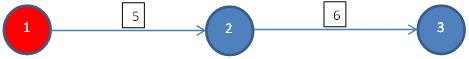
Say, at level 1 the first dimension, say x is chosen as the cutting dimension. Since we want half the points to fall on the left side and the rest half on the right side we can simply sort (typically with O(n log2(n)) complexity) he data points on x dimension and chose the middle as the root. We make sure that we remain consistent in choosing for left side points whose cutting dimension value is less than the same for root and more than or equal to for the right.

In this example, if we sort the 13 points based on the x dimension values then the root would be (5, 4). So with (5, 4) being the root at level 1, the left side points would be: (1, 3), (1, 8), (2, 2), (2, 10), (3, 6), and (4, 1). And the right side points would be (6, 8), (7, 4), (7, 7), (8, 2), (8, 5) and (9, 9). We call the tree building procedure recursively for each half data sets. We also indicate that y dimension of the data point would be chosen as the cutting dimension for the next level sub-trees.

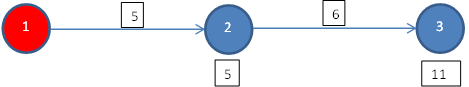
Now we have the following data points to build the left side tree with cutting dimension being y: (1, 3), (1, 8), (2, 2), (2, 10), (3, 6), and (4, 1). We can chose (3, 6) as the root, at level 2 after sorting them according to y dimension. The left side points would be (4, 1), (2, 2), and (1, 3) and the right side points would be (1, 8) and (2, 10).

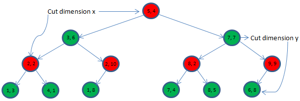
At the end the tree would look like below:

2

Bounding Box

We could visualize the points and the tree it in a different way. Let us put the 2 dimensional 13 points in x-y coordinate system.

3

The root (5, 4) at level 1 owns the whole bounding box. This root then divides the whole region into two bounding boxes: bounding box A and bounding box B, owned by second level roots (3, 6) and (8, 2) respectively.

4

Root (3, 6) would then divide the bounding box A into bounding box C and D owned by 3rd level roots (2, 2) and (2, 10) respectively. It does so using y as the cutting dimension meaning splitting the points inside A based on y dimension values.

5

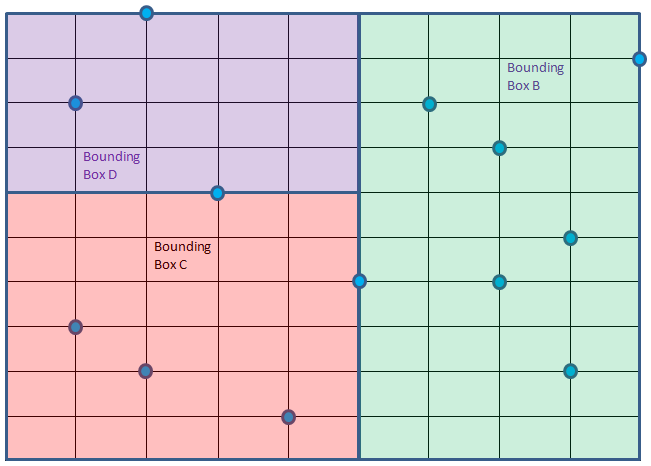
Bounding box C rooted at (2, 2) is further divided into E and F, this time using x as the cutting dimension.

6

Bounding box E can be further divided into G and H using cutting dimension y but none of them has any point. Similarly, bounding box F can be further divided into I and J using cutting dimension y, once again none of them has any point.

Bounding box D can be divided into K and L using cutting dimension x. K having one point while L having no point inside it. K is further divided into two M and N using cutting dimension y having no points left for any of them.

Similarly bounding box B will be divided into smaller boxes.

The final bounding boxes are shown below. Even though bigger bounding boxes like A is not shown here, they are all present nonetheless. Only first level division of the B bounding box is shown where (7, 7) has split it into O and P.

8

Nearest Neighbor Search

How many neighbors do we want?

We are interested to get k nearest neighbors, where k can be 1 2, 3 or any value. However, we will first see how to get the closest one point. It can then be easily extended to understand how to get more.

Points inside the same box of the query point are not necessarily the closest to query point

Suppose, we have to find the nearest neighbor of Query point Q = (4, 8) as shown below in red color. It falls inside bounding box D. But it is obvious that the closest point to Q does not fall within box D, rather it is inside Box B. Well, you can see point (6, 8) is the closest to Q. A person living near the Western border of Singapore is closer to a person living in the adjacent border of Malaysia than a person living in the eastern side of Singapore.

How to find the closest point?

We will extend the same binary search principle here. We start at root and then traverse down the tree finding the promising bounding boxes to search first and at the same time skip bounding boxes where the chance to get a closer point than the closest one to the query point found so far are thinner.

We will maintain the closest point (to Q) and minimum distance (distance between closest point and Q) found so far, at first they are null and infinite respectively. We start at root, with cutting dimension being x and do the following:

  1. If we reach a null node return.
  2. If the boundary box owned by the present root has no chance of having a point closer than minimum distance then return, meaning skip traversing that sub-tree altogether. We do so by checking the distance from Q to the bounding box. In two dimension case, it is Q to a rectangle (not a distance from Q to an actual point in the bounding box). This is how we prune search space.
  3. If the present root is closer to Q than minimum distance, we save it as the closest point and also update the minimum distance.
  4. Now we have two choices: traverse left sub-tree or traverse right sub-tree. We will compare the cutting dimension (at level 1 it is x, at level 2 it is y, at level 3 it is again x and so on) value of Q to that of root. If Q’s x is dimension value is smaller than that of root then we traverse left first, right second. So we are calling both of them but at a certain order with the hope that the first traversed sub-tree would give a closer point than any point the other side sub-tree could possibly offer. So next time when we would traverse the other sub-tree we can do a quick check and completely skip traversing that sub-tree. Something that might not materialize as well.

9

Let us walk through this particular example. At root (5, 4), closest point so far is null, minimum distance is also null. We set the root as the closet point and minimum distance (using commonly used Euclidean distance for continuous values) to ((x1 – x2)2 + (y1 –y2)2)1/2 = 4.12 (approx.). Now we have two bounding boxes A and B. The decision that we need to make is which one to traverse first? Q’s x dimension value 4 is smaller than root’s x dimension value that is 5. So we choose left first, right second. Both of them are to be called by using the cutting dimension y. The bounding box for each of the call is going to change. Well, we know each root owns a bounding box.

At the second call, root is (3, 6), bounding box is A. Distance from Q to A is zero as Q is within A. So we cannot skip traversing this sub-tree. Distance from (3, 6) to Q (4, 8) is 2.24, closer than existing minimum distance 4.12. Hence, we update our closest point to (3, 6) and minimum distance to 2.24. Next decision to make is again which side to traverse first. We have Q’s y value 8 that is more than present root’s y value 6. So we will traverse the right side first, left side second.

Next, the function is called with root, (2, 10), cutting dimension x and bounding box D. Distance between (2, 10) and Q (4, 8) = 2.83 that is larger than existing minimum distance. So we are not updating the closest point in this call. Next – choose which side to traverse first. Q’s x dimension 4 is bigger than root’s x dimension 2, hence right sub-tree is chosen first that is null anyway. So the call to it will return without doing anything.

Next call would be made with root (1, 8) that is 3 units away from Q. No improvement for the closest point. Also this root has no children. We have reached bottom of this side of the tree in our DFS search.

Next call is done with root (2, 2), far away from Q. But the bounding box owned by it is only 2 units away from Q. Hence, there is a chance that we might end up getting a closer point from this area. Hence, we cannot skip this tree. Right side to traverse first based on x dimension value comparison.

Root (4, 1), that is 8 units away from Q is called. It owns bounding box F that is 2 units away from Q. Once again cannot skip this area. Well, it has no child anyway.

Root (1, 3) is called that owns bounding box E that is 2.83 units away from Q, having no chance to offer any closer point. For the first time we can skip this area/sub-tree/bounding box.

We are done with the left side of level 1 root (5, 4). Now traverse right side.

Sub-tree with root (7, 7) owing bounding box O is called. Subsequently sub-tree rooted at (6, 8) would be called and that would be the closest point at distance 2.

How much search space did we prune?

We will skip traversing the left sub-tree rooted at (8, 2) that owns bounding box P. In terms of nodes we skipped only 4 nodes, 3 of them are rooted at (8, 2). Previously we skipped sub-tree rooted at (1, 3) as well. The green areas were pruned, meaning we did not search there. That was not quite efficient though!

10

How to get k nearest neighbors?

Instead of keeping a single closest point we could maintain a priority queue (max heap) to keep k (say 2, 3 or any number) closest points. The first k points would be en-queued anyway. Onwards, a new point, if better, would replace the worst of the closest point found so far. That way we can maintain the k nearest points easily.

Too few points is a problem

If we have to construct a k-d tree with 20 dimensional data sets, we got to have around 220 data points. If we don’t have enough data then at many levels we will not have sufficient data to split. We will also end up with an unbalanced k-d tree where search and other operations would not be very efficient.

In general, we need k-d tree when we have higher dimensional data points. But when the dimension is too high other approaches might work better.

Index

Bellman-Ford Algorithm

17th Friday Fun Session – 12th May 2017

We use Bellman-Ford Algorithm to find the shortest path from a single source node/vertex (red color) to all destination nodes/vertices.

Let’s use our intuition

Image1

Given that distance from city-1 (city-1 is node 1 here) to city-2 is 5, and from city-2 to city-3 is 6, if I have travel from city-1 to city-2 and city-3 respectively what would be the cheapest way to do so?

We can start from city-1 and reach city-2 at cost 5. Now that we have arrived at city-2 at cost 5, we can add cost 6 to it and reach city-3 via city-2. Thus, the shortest path from city-1 to city-2 and city-3 are respectively 5 and 11.

Image2

Distance

Since city-1 is the source, we can add a self-loop on it with cost 0. That means, reaching city-1 from itself would cost 0. We also set that reaching city-2 and city-3 would cost infinity. We set so, because as of now we don’t know what would be the cost to reach there. So we put the maximum possible cost. Let’s call it distance. So we have distance [1] = 0, distance [2] = ∞ and distance [3] = ∞.

Predecessor

Let’s also maintain another array, called predecessor to indicate the last node from which we arrived here. We set predecessor [1] = 0, predecessor [2] = 0, predecessor [3] = 0.  Since we have not arrived to city-2 and city-3 yet, we set the predecessor value for them to something invalid (0). For city-1, it is the source, can be set to 0 as well.

Relaxation

Now we take each path/edge. We have two edges here. First one is from city-1 to city-2 with cost 5 and the second edge is from city-2 to city-3 with cost 3. Now let’s do what is called relaxation on each of the edges.

We see that using first edge we can arrive at city-2 from city-1 at a cost of 5 (distance [1] + cost of first edge). Since 5 is less than the existing distance of city-2 that is ∞, we update distance [2] to 5. We also note that, we arrived here from city-1 and hence got this new distance, that means we also update predecessor [2] = 1.

Now let’s do relaxation on edge 2. We see that distance [3] that is ∞ as of now can be improved by using edge 2. We set distance [3] = distance [2] + cost of edge 2 = 5 + 6 = 11. Since we arrived here from city-2, let’s update predecessor [3] = 2.

Does order of edges for relaxation matter?

Now we are done with relaxation for all the edges once. First, we did the relaxation on first edge. Then we did the relaxation on the second edge. What would happen if the we changed the order? That means do the relaxation on the second edge first and then do it on the first edge.

Let’s do it. Start the relaxation afresh with new edge order. As of now we have predecessor [1] = 0, predecessor [2] = 0, predecessor [3] = 0. Also distance [1] = 0, distance [2] = ∞ and distance [3] = ∞.

We do relaxation on second edge (city-2 to city-3 at cost 6) first. We see that both distance [2] and distance [3] = ∞. Hence there is no chance to improve distance [3] since distance [2] + 6 = ∞ + 6 = ∞, that is no better than the existing distance [3] that also ∞. Hence relaxing second edge did not yield anything.

Let’s do relaxation on first edge. We know that would result in distance [2] = 5 and predecessor [2] = 1.

Well, at this point we see that we are done with relaxation on all the edges once and yet we have not found the shortest path to reach city-3.

So when shall we get the result?

Iteration

That brings us to the next concept called iteration. Relaxation on all the edges once is called an iteration. So how many iterations do we need to get the shortest path to all destination nodes? Let’s use our intuition on the example that we are working on. We got 3 nodes. So if we have to reach from one end (say node 1) to the other end (say node 3), the maximum edges we might have to travel is 2, that is, the number of nodes minus 1. If we do the relaxation on the edges in an order that would choose the furthest edge from source (or the closest to the destination, in this case, second edge that is going from city-2 to city-3 at cost 6), we see that at each iteration we would increase the path (source node to furthest node) by at least one edge. And hence at 2 iterations we will certainly reach all reachable (I am saying reachable because all destinations might not be reachable) destinations.

Let’s continue our workout from where we left. Let’s start iteration 2 for the cases when we did the relaxation on second edge first. At this 2nd iteration, we again start with second edge. This time we can update distance [3] = distance [2] + 6 = 5 + 6 = 11. Predecessor [3] = 2.

We are done with2 iterations and we have found the result to reach from city-1 to both city-2 and city-3.

Are all nodes reachable?

Let’s consider the below example, that is constructed by adding one more node 4.

Image3

We will see that distance [4] will remain ∞ and predecessor [4] will remain 0 (invalid) after |V| -1 = 4 – 1 = 3 iterations, where |V| is the number of nodes/vertices. This is because there is no incoming edge (path) to city-4. Hence city-4 is unreachable.

Did order of edges for relaxation really matter?

We have seen that intermediate results (distance and predecessor values) might vary based on the order of edges we chose for relaxation but final result after all the iterations will still be the same. Hence the order of edges on which we do relaxation does not really matter (as far as final result is concerned).

So after |V| – 1 iterations we have got the correct result?

Unfortunately not! Well, we did get the final result. But as of now we don’t know whether the result is valid or not. That sounds interesting. So, we have found the result and still we don’t know whether the result is correct/valid or not. So what is the issue? Well, let’s consider the below case.

Image4

I have added a third edge from city-3 to city-1. And the cost is -12. Negative cost? Why? We don’t answer the why question but let’s answer the what question. Cost -12 means reaching city-1 from city-4 would cost -1.

Let’s continue our workout where we have finished 2 iterations by considering the second edge first. Let’s assume we also considered the third edge and that third edge was considered at first for relaxation at each iteration. Distance [3] got a less than infinity value after 2nd iteration. Since we used 3rd edge at first, that means third edge was not used till 2nd iteration to update any distance for any node. That means the values (distance and predecessor) we got last time would be the same value even with the presence of third edge after 2 iterations.

Since we just added an extra edge (3rd edge) but no new nodes, the number of iterations we have to do still remains 2. That also means the result we found so far still valid in this case. But is the result (distance [2] = 5 and distance [3] = 11) correct with this new situation?

Negative cycle

Now that you arrived at city-3 at cost 11, you can go to city-1 at cost 11 + (-12) = -1 and then city-2 at -4 and so on. The more you travel, the less cost you would incur. And hence the shortest path found after 2 iterations are not valid.

So how do we find that the result is invalid? Well after we are done with |V|-1 iterations, we have to do one more iteration that is the |V|th one (a cycle involving |V| nodes can be found with |V| edges). If that changes distance value for any node that means there exists a negative cycle (a cycle whose edges (costs) sum to a negative value). When there is negative cycle present in a graph then the answer found is invalid.

Negative edge vs. negative cycle

Does negative edge means negative cycle? Does presence of negative edge mean no answer can be found?

Image5

Negative edge is fine with Bellman-Ford as in the above example. A correct solution can still be found. A correct solution cannot be found when there is a negative cycle. But Bellman-Ford can detect a negative cycle and in that case it can indicate that a correct solution is not found.

Are all iterations required?

Not really. When we did the relaxation on the first edge first, we already found the shortest paths to both city-2 and city-3. How do we know? Well, at iteration 2 we would have found that no distance got updated. If an iteration does not change any distance value then we can terminate the algorithm there and return valid result. Because in that case, subsequent iterations are not going to change anything. It also means there is no negative cycle.

The shortest path sequence

We can use the predecessor array recursively to get the shortest path sequence. For example, earlier after 2 iterations we got the following result.

distance [1] = 0, distance [2] = 5, distance [3] = 11

predecessor [1] = 0, predecessor [2] = 1, predecessor [3] = 2

If we want to find the shortest path sequence to city-3, we can find the predecessor [3] that is 2, recursively we can check the predecessor [2] that is 1 and that equals to source node, that is city-1. So we stop and the sequence is city-1 to city-2 to city-3.

Distance for a particular node can be updated more than once in an iteration

Image6

In this example above we have two nodes. We have to do one iteration. We have two edges: first with cost 5, second with cost 2. Source is node 1. If we relax the first edge then distance [2] will be 5. Subsequent relaxation on second edge would result the node 2 distance to be updated again with 2 (because, existing distance 5 > (0 + 2)). We see that node 2 distance got updated twice within the same iteration.

The algorithm

Now that we have done with the workout, let’s write down the algorithm.

Function BellmanFord()
{
  input = G {V, E};
  distance[] = ∞;
  predecessor[] = -1;
  distance[sourceNode] = 0;

  for i = 1 to |V|-1
  {
    valueChanged = false;
    for j = 1 to |E|
      valueChanged = Relax (E[j]) || valueChanged;

    if(!valueChanged)
      return Result();
  }

  for j = 1 to |E|
    if(Relax(E[j])
      print ‘negative cycle detected, solution not possible’;
}

Function Relax (e)
{
  if(distance[e.to]) > distance[e.from] + e.cost)
  {
    distance[e.to] = distance[e.from] + e.cost;
    predecessor[e.to] = e.from;
    return true;
  }

  return false;
}

Function Result()
{
  print ‘success’;
  print distance[];
  print predecessor[];
}

The complexity

For each iteration (number of vertices – 1), we are iterating over all the edges. That means the complexity is O(|V|. |E|).

GitHub: Manipulating Money Exchange

Index

Friday Fun Session

At JLTi, I conduct an half an hour learning session every Friday from 5:30 PM to 6:00 PM. It is regularly attended by 10 to 20 enthusiastic engineers from JLTi Singapore and Mumbai office and a few from JLT Regional IT. We call it Friday Fun Session.

We started it from Jan 2017 and so far we made it every week except few when we missed it dearly due to public holiday etc.

As of we now we discuss data structure, algorithm, and machine learning among others.

For every Friday Fun Session, I will also post a blog.

I am also creating a group beyond JLTi with like-minded enthusiastic lifelong learners. In future, we might organize a regular tech meetup!

If you are outside JLTi and interested to join this journey please write to me. I would be very glad to include you in our learners’ family.

And finally, thank you all so much who participate in the session, and encourage me to continue it. It is only you who made it a success so far.

Complete list of topics covered so far.

Making Money at Stock Market

3rd JLTi Code Jam – May 2017

Input: price = [961, 984.5, 965, 988.5, 956.5]

Explanation: Now that your bank accounts are flooding with April bonus money and you are contemplating to invest in stock market why not join me in doing some analysis first? After all, we are engineers flooded with data (quite a lot of them are free) and the capability to analyse them. I opened JLT’s historical stock price from yahoo finance. It’s amazing! As part of the analysis, you know, we have to do a tremendous amount of work. As a start, I wanted to focus on when to buy and when to sell a stock so that I can make the most profit. For example, I took the data from 19th Dec 2016 to 23rd Dec 2016 as specified above. I did some manual calculation and found that had I bought on 19th Dec 2016 at £961 and sold on 22nd Dec 2016 £988.5, I could make the most profit, £27.5.

I also checked if I had to make the most profit by buying and selling a single JLT share once within 2016 , I could do so by buying on 9th Feb 2016 at £776.5 and selling on 11th Apr 2016 at £1070, making a whopping £293.5 profit! I have not put the data here as one year’s data is too huge to fit here. You can collect and verify it by downloading it as an excel file from the above yahoo link.

Output: Buy on day 1 at £961 and sell on day 4 at £988.5, making £27.5

I also checked the values from 15th Jan 2016 to 21st Jan 2016 (excluding 16th Jan 2016 and 17th Jan 2016 when stock market was closed) and the price looked like the below.

Input: price = [890, 890, 853.5, 828.5, 809]

You can see it kept on dropping and there was no way to make money in this period.

Output: Don’t buy stock

Task: As you realize, as part of the bigger data analysis work that we need to do, it is a small part. We got so much data for hundreds of companies. Hence, it is essential that we do it efficiently. To be precise, I am looking for a solution more time efficient than O(n2).

Index

No Two Team Members Next to Each Other

1st JLTi Code Jam – Mar 2017

Input: 1, 1, 2, 2, 2, 567, 567, 10000076, 4, 2, 3, 3

Explanation: There are 12 people listed above. They belong to 6 teams (Team 1, Team 2, Team 3, Team 567, Team 10000076, and Team 4). As you can see people are identified in the list by the team number.

Output: 1, 2, 1, 2, 4, 2, 567, 3, 567, 100076, 2, 3

As you can see, the output has rearranged the team members in way that no two members from the same team standing next to each other.

Input: 1, 1, 1, 1, 2

Output: It is not possible to rearrange them.

Task: You have to write a program that can rearrange even billions of such team members belonging to millions of teams very fast. If the input is such that it is not possible to rearrange then the output should be: It is not possible to rearrange them. A correct solution is not sufficient. The algorithm has to be efficient, otherwise the output for big data 🙂 will not come.

GitHub: No Two Team Member Next to Each Other

Index

Company Tour 2017 to Noland

2nd JLTi Code Jam – Apr 2017

Input: Capacity = 125, w = [45, 25, 80, 100, 125]

Explanation: This year, RC has taken all JLT Asia employees to Noland for the company trip. As the name implies there is not much land in Noland, it is river everywhere. When we have to cross such a river having only one boat with a certain capacity (in the above example 125 Kg), Warren Downey, our Deputy CEO approaches RC and asks us to quickly divide the people so that each trip of the boat carries people exactly to its maximum capacity, 125 Kg in this example. He shows the example above and works out the below output that he desires.

Output: {45, 80}, {25, 100}, {120}

When RC team pointed out what would happen for a scenario when we have a case like Capacity = 120, w = [40, 20, 80, 100, 120, 70]. Warren informs us we always utilize our resources to its maximum capacity. No compromise. We will not cross the river and will change the tour itinerary.

Output: No crossing, change itinerary.

Task: When I woke up an hour ago from my afternoon nap with a lot of stress, I realized that the tour was just a bad dream. I started feeling relaxed. But the problem got into my head and now it is itching everywhere inside it. In this situation, I realize, I can spread the itching to my JLTi friends in Singapore and Mumbai as well.

You can imagine there is a boatman and his weight is out of consideration. The input capacity is only applicable for the passengers. The input w array is holding only the passenger weights. In short, you can ignore the boatman.

GitHub: Company Tour to Noland

Index