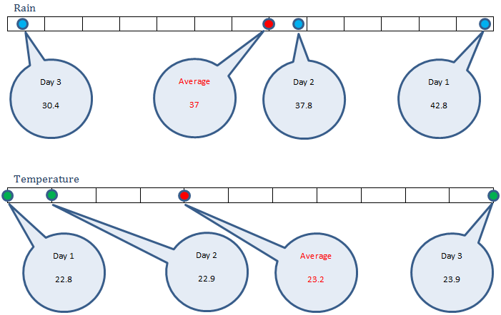
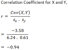
15th Friday Fun Session (Part 1) – 28th Apr 2017
Usually, machine learning algorithms build a model. We are trying to understand what a model looks like and some associated concepts around it.
Descriptive vs. predictive analytics
Descriptive analytics looks at historical data to understand what happened. It describes historical data using different statistical techniques and visualization.
Predictive analytics looks at historical data to understand and predict future. It also uses different statistical techniques, machine learning algorithms etc.
Both can have models, called as descriptive and predictive models. Here by model we are referring to predictive model.
Understanding model
The globe of the Earth does not show every detail of it but this small model can be put on our desk and it can give us an idea as to how the Earth looks like. When we talk about machine learning model, it is similar to that. It represents the data that is used to build it.
Suppose we have some employee data as shown in the table below.

We want to build a model using this data set. Later, given an employee’s salary and experience, we would like to know her designation, using it.
Model as logical statement or rule
Based on the above data, we can construct two logical statements as shown below.
If salary is more than 3,000 and experience is more than 5 years
then the employee is a Senior Software Engineer.

Otherwise, the employee is a Junior Software Engineer
Given an employee’s salary and experience, we can find her designation by using the above formula. That formula is called the model.
Model as function
The formula can take the form of a function as well. Let us draw a function that can work as a model for the above data set.
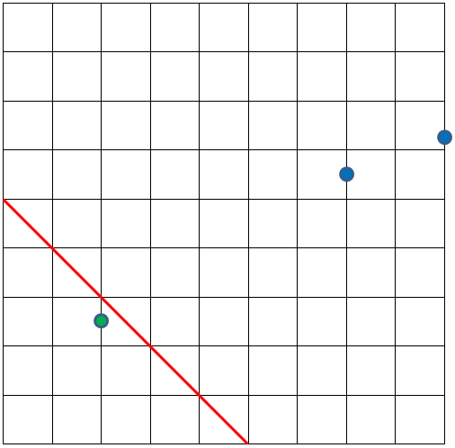
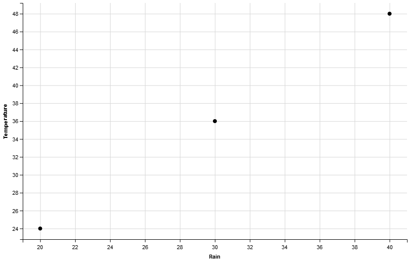
We have used X-axis for experience, and Y-axis for salary (in thousands). The three data points would be placed as shown above.
The red line can work as a model. All employees on the left side of it, shown as green points are Junior Software Engineers. And all employees on the right side of it, shown as blue points, are Senior Software Engineers.
Note that, this model is not an exact translation/equivalent of the earlier model expressed as logical statements. Meaning, the same input data might be classified (Junior Software Engineer or Senior Software Engineer) differently.
The (red) line equation can be written as
   x + y = 5
=> x + y - 5 = 0
=> f(x, y) = x + y - 5

The model can be expressed this way:
if f(x,y) >= 0, then Senior Software Engineer
if f(x,y) < 0, then Junior Software Engineer
If a new employee input comes with salary 4,500, and experience 1 year, this model would classify her as a Senior Software Engineer.
   f(x, y) = x + y - 5
=> f(x,y) = 4.5 + 1 - 5
=> f(x,y) = 0.5
=> f(x, y) >= 0
If we use the earlier model to classify this input, it would classify it as Junior Software Engineer – different prediction!
Hybrid model
A model can use a combination of both logical statement and function.
To summarize, a model can be expressed using logical statement, function or a hybrid of both.
When a model is built?
At the beginning when we have some data, usually we split it into training data and test data; we provide the training data to a machine learning algorithm that in turn builds a model. Then we use the test data to check how this model is performing and tune the model, as and if required. The model can be further updated, say, periodically, when more data is gathered.
Different machine learning algorithms build different kinds of model. Some build at first, some delay it.
Eager vs. Lazy learning
When a machine learning algorithm builds a model soon after receiving training data set, it is called eager learning. It is called eager; because, when it gets the data set, the first thing it does – build the model. Then it forgets the training data. Later, when an input data comes, it uses this model to evaluate it. Most machine learning algorithms are eager learners.
On the contrary, when a machine learning algorithm does not build a model immediately after receiving the training data, rather waits till it is provided with an input data to evaluate, it is called lazy learning. It is called lazy; because, it delays building a model, if it builds any, until it is absolutely necessary. When it gets training data, it only stores them. Later, when input data comes, only then it uses this stored data to evaluate the result.
There is a different set of pros and cons associated with eager and lazy learning. It is obvious that lazy learning would take less time during training but more time during prediction.
Eager learning builds a model for the whole data set, meaning it generalizes the data set, at the beginning. It might suffer accuracy compare to lazy learning that has more options in terms of the availability of the whole data set as well as the mechanisms to make use of it.
Lazy learning is typically divided into two types: instance-based learning and lazy Bayesian rules.
Instance-based learning
Do all machine learning algorithms build a model?
No, all machine learning algorithms don’t build a model, when by model we mean generalizing the data. For example, decision tree builds a model but k-NN does not.
A row is also called an instance, meaning a set of attributes. Hence a set of training data is also called a set of instances. When a machine learning algorithm does not build a model, rather uses the set of instances directly to evaluate the result, it is called instance-based learning. It is also called memory based learning as it memorizes the whole data set. For the same reason it is also called rote learning.
Instance-based learning, as mentioned above is one kind of lazy learning.
Supervised, unsupervised and semi-supervised learning
The employee example that we have discussed here is an example of supervised learning. Here we wanted to predict an output variable – designation of an employee by providing input variables – salary and experience. While building the model, we provided training data having most (all for the example here) values for input variables and all values for the corresponding output variable.
An important requirement of supervised learning is that, for all the training data we must provide the output variable value. Because, supervised learning learns from it. Most machine learning algorithms use supervised learning.
However, some machine learning algorithms don’t predict an output variable. They just take only the input variables and try to understand, say the distribution or pattern of the data. They are classified mainly into clustering and association rules. For example, when we do clustering, it might come up and say the given data falls into 3 groups.
There is a third type of learning, in the middle of supervised and unsupervised, called semi-supervised. In many real life examples, a good portion of the training data does not have labels for the target variable, meaning many instances of the training data don’t have the output attribute value known. It might be expensive to label them as it might require domain experts.
In this situation, unsupervised learning comes to rescue. It labels them, and then the labelled data is fed into supervised algorithm (to build model) for prediction. This process (unsupervised algorithm labels them and supervised algorithm predicts), might be repeated unless satisfactory accuracy is acquired.
In the above example, we have seen examples of supervised models. However, predictive models include unsupervised and semi-supervised models as well, the latter being a combination of supervised and unsupervised models.
Parametric vs. non-parametric model
Some machine learning algorithms would come up with a model with a predetermined form. For example, it would construct a function with 2 parameters. Now given the training set it would compute that two parameters and come up with a function. An example would be naive Bayes. They are called parametric. For prediction they would depend on this function alone.
On the other hand, some machine learning algorithms would construct a model based on the information derived from the data. For example, k-NN, C4.5 – a decision tree etc. They are called non-parametric. Non-parametric does not mean no parameter, rather no predetermined parameters.
k-NN as an example of a non-parametric model might create a little confusion as k-NN does not build any model at the first place. Well, here model is used in a broader sense to mean how it computes output value. K-NN uses the complete training data set to do so. Hence the whole training data set is the input parameter. Adding one more training data can be thought as increasing the parameter by one. That perfectly matches another definition of non-parametric model that says – the number of parameters grows with the amount of training data.
Classification vs. regression
The model that we are discussing so far – given salary and experience, predict the designation, is called a classification model. The reason is the output variable, designation – a categorical variable. Meaning, it would take one of the predefined categories or classes. In this example, there are two categories or classes: Junior Software Engineer and Senior Software Engineer.
Let us alter the input and output a bit for the model. Suppose the model would now predict the salary, given experience and designation. Then this model would be called a regression model. The reason is the output variable, salary – a continuous variable. Meaning, it can take any value, not limited by a predefined set of classes, unlike earlier example.
Bias vs. variance
Let us continue with the previous example of the model that predicts salary. Ideally, the salary would be calculated by taking the input values, experience and designation into consideration.
But assume the model that is built by a machine learning algorithm, is so simple and dumb. Let us say, given the training data, it computes the average of the salary (2500 + 5500 + 6200) / 3 = 4733 by ignoring all other parameters. Now when an input comes asking the salary, it does not care the experience or designation of the input. The only output (salary) that comes out of it is 4733. Now that is called a highly biased model. It generalizes the data so much that it ignores the input values of the training data and hence underfits the training data. A biased model that does not distinguish a 2 years experienced Junior Software Engineer from a 15 years experienced Senior Software Engineer, and predicts the same salary of 4733 for both, is not a good model, for obvious reasons.
By the way, what machine learning algorithm can possibly come up with such a model and under what condition?
On the other extreme, there is this model with high variance that considers each minute detail of the training data that is possibly nothing but noise, to be the ultimate truth and incorporates them into the model. Hence it is said to be overfitting the training data, and results in a highly complex model. However, a model with all these intricate truths of training data, even though performs very well with training data (after all, the model is built to overfit the training data), do not stand the test of real world. This kind of model, with highly fluctuating prediction, due to little changes in input parameters, is not desirable either.
What we need is a balance, a trade-off between bias and variance; achieving which is a prerequisite, for a good model.