Currency Arbitrage with Decreasing Rate

12th JLTi Code Jam – Feb 2018

Here we extend the Currency Arbitrage problem that expected us to re-compute the best path cost matrix when a new currency arrived along with some rates from and/or to the existing currencies. We came up with a solution at O(n2) cost.

If we look at the currency exchange issues, we realize that new currencies are not arriving every day. Rather, rates among the existing currencies are the ones which are changing every now and then. So it’s equally, if not more, important to find a solution as to how to address the rate changes and compute the cost matrix.

Rate between two currencies can either increase or decrease. Here we will focus only on rate decrease.

Given that we have an existing best path cost matrix, when a rate between two currencies decreases what shall we do? Well, just like Currency Arbitrage problem, we have two options:  i) re-compute the cost matrix from the scratch, using Floyd-Warshall, at a cost O(V3) and ii) update the already computed cost matrix using some partial computations. This problem expects a solution using the second option.

Input:

1 USD = 1.380 SGD

1 SGD = 3.080 MYR

1 MYR = 15.120 INR

1 INR = 0.012 GBP

1 GBP = 1.30 USD

I CAD = 0.57 GBP

1 GBP = 1.29 USD

Explanation: We have 7 inputs here. Each time an input is given, we need to present an output and hence, we have 7 lines of output. We already know how to incrementally add a new currency. The first 4 do not result in any arbitrage; we output “No luck here”. For 5th, we have an arbitrage and we output the same. For 6th, we continue to have the same arbitrage and we again output the same.

At 7th input, we see the existing rate from GBP to USD, which was 1.30 last time, has changed to 1.29 now. With this new rate in effect, the arbitrage disappears now. Output should be “No luck here”.

Since we are dealing with only decreasing rate, in input, between two currencies, rate will only decrease. For example, an input like 1 GBP = 1.31 USD will never appear.

When multiple arbitrages exist, printing any one will do.

Output:

No luck here

No luck here

No luck here

No luck here

USD -> SGD -> MYR -> INR -> GBP -> USD

USD -> SGD -> MYR -> INR -> GBP -> USD

No luck here

Task: For each line of input, for each new vertex, incrementally adjust/add shortest paths at a cost (time) of O(|V|2), detect the presence of an arbitrage and output as specified. Use existing solution for this.

If input contains a rate that decreases since last time, accommodate that change in the best path cost matrix using some partial computations, instead of computing the whole matrix from the scratch.

Index

Solution – Currency Arbitrage

49th Friday Fun Session – 2nd Feb 2018

Negative Cycle can be identified by looking at the diagonals of the dist[][] matrix generated by Floyd-Warshall algorithm. After all, diagonal dist[2][2] value is smaller than 0 means, a path starting from 2 and ending at 2 results in a negative cycle – an arbitrage exists.

However, we are asked to incrementally compute the same, at cost of O(n2) for each new vertex.

Floyd-Warshall algorithm takes O(n3) time to compute All-Pairs Shortest Path (APSP), where n is the number of vertices. However, given that it already computed APSP for n nodes, when (n+1)th node arrives, it can reuse the existing result and extend APSP to accommodate the new node incrementally at a cost of O(n2).

This is the solution for JLTI Code Jam – Jan 2018.

Converting Rates

If USD to SGD rate is r1 and SGD to GBP rate is r2, to get the rate from USD to GBP, we multiply the two rates and get the new rate that is r1*r2. Our target is to maximize rate, that is maximizing r1*r2.

In paths algorithm, we talk about minimizing path cost (sum). Hence maximizing multiplication of rates (r1*r2) would translate into minimizing 1/(r1*r2) => log (1/(r1*r2))  => log (r1*r2) -1 => – log r1 – log r2 => (–log r1) + (–log r2) => sum of (–log r1) and (–log r2). Rate r1 should be converted into – log r1 and that is what we need to use in this algorithm as edge weight.

While giving output, say the best rate from the solution, the rate as used in the dist[][] matrix should be multiplied by -1 first and then raised to the bth power, where b is the base (say one of 2, 10 etc.) of the log as used earlier.

Visualizing Floyd-Warshall

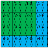
We have seen the DP algorithm that Floyd-Warshall deploys to compute APSP. Let us visualize to some extent as to how it is done for 4 vertices.

What Cells Are Used to Optimize

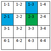
The computation will be done using k = 1 to 4, in the following order – starting with cell 1-1, 1-2, . . . . .2-1, 2-2, …….3-1, ……. 4-3, 4-4.

At first, using k = 1.

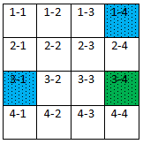
Let us see how the paths are improving using the following two examples.

dist[2][3] = min (dist[2][3],  dist[2][1] + dist[1][3])

1

and dist[3][4] = min (dist[3][4],  dist[3][1] + dist[1][4])

2

We see that for k = 1, all paths are optimized using paths from 1st (kth) row and 1st (kth) column.

Kth Row and Column do not Change

What about paths on kth row and kth column?

dist[1][2] = min(dist[1][2], dist[1][1] + dist[1][2]) – well, there is no point in updating dist[1][2] by adding something more to it.

So we see, at a certain kth iteration, kth row and kth column used to update the rest of the paths while they themselves are not changed.

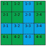
At k = 1

3

At k = 2

4

At k = 3

5

At k = 4

6

Consider Only 3X3 Matrix Was Computed

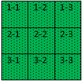
Now assume that we did not consider that we had 4 vertices. Rather we considered that we had 3 vertices and completed APSP computations for all paths in the 3X3 matrix. We ignored the 4th row and column altogether.

So we have APSP computed for the following matrix using k = 1, 2 and 3.

7

Add 4th Vertex

Let’s say, 4th vertex arrives now. First, we can compare the computations used for the above 3X3 matrix with the same for the 4X4 matrix as shown earlier and find out what all computations need to be done now to extend this 3X3 matrix to 4X4 matrix to accommodate the new 4th vertex.

We will find that at first we have to optimize the 4th row and column using k = 1, 2 and 3. Let us do that.

8

Note that at this point, 4th row and column are not used to optimize paths for the older 3X3 matrix. So now that we have the 4th row and column optimized using k = 1, 2 and 3, we have to optimize that 3X3 matrix using k = 4.

9

This way, we don’t miss out any computation had we considered all the 4 vertices at one go. And thus we are done with optimizing all the paths in the 4X4 matrix.

Code

dist[][] //APSP matrix, already computed for n-1 vertices

p[][] //predecessor matrix, already computed for n-1 vertices


dist[n][] = ∞

dist[][n] = ∞

dist[n][n] = 0


for each edge (i, n)

  dist[i][n] = weight(i, n)

  p[i][n] = n


for each edge (n, i)

  dist[n][i] = weight(n, i)

  p[n][i] = i


for k = 1 to n-1

  for i = 1 to n-1

    if dist[i][n] > dist[i][k] + dist[k][n]

      dist[i][n] = dist[i][k] + dist[k][n]

      p[i][n] = p[i][k]

  for j = 1 to n

    if dist[n][j] > dist[n][k] + dist[k][j]

      dist[n][j] = dist[n][k] + dist[k][j]

      p[n][j] = p[n][k]


for i = 1 to n-1

    for j = 1 to n-1

      if dist[i][j] > dist[i][n] + dist[n][j]

        dist[i][j] = dist[i][n] + dist[n][j]

        p[i][j] = p[i][n]

Complexity

The complexity for this incremental building for a new vertex is clearly O(n2). That makes sense. After all, for n vertices the cost is O(n3) that is the cost of Floyd-Warshall, had all n vertices were considered at one go.

But this incremental building makes a huge difference. For example, consider that we have 1000 vertices for which we have already computed APSP using 1 billion computations. Now that 1001st vertex arrives, we can accommodate the new vertex with a cost of 1 million (approx.) computations instead of doing 1 billion+ computations again from the scratch – something that can be infeasible for many applications.

Printing Arbitrage Path

We can find the first negative cycle by looking (for a negative value) at the diagonals of the dist[][] matrix, if exists and then print the associated path. For path reconstruction, we can follow the steps as described here.

GitHub: Code will be updated in a week

Index

Dijkstra’s Algorithm

10th Friday Fun Session – 17th Mar 2017

Dijkstra’s algorithm is a Single-Source Shortest Path (SSSP) algorithm developed by Edsger Wybe Dijkstra. It uses a greedy process and yet finds the optimal solution. It looks similar to Breadth-first search.

Compare to Bellman-Ford

It is asymptotically the fastest SSSP algorithm, at a cost O(|E|+|V|log|V|), when min-priority queue implemented by Fibonacci heap is used.

That is quite cheap, given Bellman-Ford’s complexity of O(|V||E|) to find the same, something that can become prohibitively expensive for a dense graph having |V|2 edges.

However, while Bellman-Ford can work with negative edge and can detect negative cycle, Dijkstra’s algorithm cannot work with negative edge. Since it cannot work with negative edge, there is no question of detecting negative cycle at all.

Standard Algorithm

dist[] //shortest path vector

p[] //predecessor vector, used to reconstruct the path

Q //vertex set

for each vertex v in Graph
  dist[v] = ∞
  p[v] = undefined
  add v to Q

dist[s] = 0

while Q is not empty
  u = vertex with min dist[] value
  remove u from Q

  for each neighbor v of u
    alt = dist[u] + weight(u, v)
    if alt < dist[v]
      dist[v] = alt
      p[v] = u

return dist[], p[]

Given source vertex s, it finds the shortest distance from s to all other vertices. At first, it initializes dist[] vector to infinite to mean that it cannot reach any other vertex. And sets dist[s] = 0 to mean that it can reach itself at a cost of 0, the cheapest. All vertices including itself are added to the vertex set Q.

Then, it chooses the vertex with min dist[] value. At first, s (set to u) would be chosen. Then using each of the outgoing edges of u to v, it tries to minimize dist[v] by checking whether v can be reached via u using edge (u, v). If yes, dist[v] is updated. Then again it retrieves vertex u with the cheapest dist[u] value and repeats the same. This continues till Q is not empty. Whenever, a vertex u is removed from Q, it means that the shortest distance from s to u is found.

Since we are retrieving |V| vertices from Q, and for each vertex, trying with all its edges (=|V|, at max), to minimize distance to other vertices, the cost can be |V|2.

So, here we see a greedy process where it is retrieving the vertex with min dist[] value.

Since retrieving a vertex u from Q means that we found the minimum distance from s to u, if we are solving shortest path from a single source s to a single destination d, then when u matches the destination d, we are done and can exit.

It can also be noted that from source s, we find the shortest distances to all other vertices, in the ascending order of their distances.

Finally, we see that dist[] vector is continuously changing. And each time when we retrieve a vertex u, we choose the one with min dist[] value. That indicates using min-priority queue might be the right choice of data structure for this algorithm.

Using Fibonacci Heap

dist[] //shortest path vector
p[] //predecessor vector, used to reconstruct the path
Q //priority queue, implemented by Fibonacci Heap

dist[s] = 0

for each vertex v
  if(s != v)
    dist[v] = ∞
    p[v] = undefined
  
  Q.insert_with_priority(v, dist[v]) // insert

while Q.is_empty() = false
  u = Q.pull_with_min_priority() // find min and delete min
  
  for each neighbor v of u
    alt = dist[u] + weight(u, v)
    if alt < dist[v]
      dist[v] = alt
      p[v] = u
      Q.decrease_priority(v, alt) //decrease key

return dist[], p[]

In the above algorithm, we have used a function called decrease_priority(), something that is absent in standard priority queue but present in Fibonacci heap. So the above algorithm is implemented using Fibonacci heap.

Fibonacci heap is a special implementation of a priority queue that supports decrease key (decrease_priority()) operation. Meaning, we can decrease the value of a key while it is still inside the priority queue. And this can be achieved by using constant amortized time for insert, find min and decrease key operation and log (n) time for delete min operation.

As for cost, since we have called delete operation for each of the v vertices, and we have treated each of the |E| edges once, the cost here is O(|E|+|V|log|V|), as mentioned at the beginning of this post, as the cost of Dijkstra’s algorithm.

Using Standard Priority Queue

Standard priority queue implementation takes log (n) time for both insert and delete operation and constant time for find min operation. But there is no way to change the key value (decrease key) while the item is still in the priority queue, something Dijkstra’s algorithm might need to do quite frequently as we have already seen.

If standard priority queue is used, one has to delete the item from the priority queue and then insert into it again, costing log (n) each time, or an alternative to that effect. However, as long as standard priority queue is used, it is going to be slower than Fibonacci heap. With standard priority queue, the algorithm would look like below:

dist[] //shortest path vector
p[] //predecessor vector, used to reconstruct the path
Q //standard priority queue

for each vertex v
  dist[v] = ∞
  p[v] = undefined

dist[u] = 0
Q.insert_with_priority(u, dist[u]) // insert

while Q.is_empty() = false
  u = Q.pull_with_min_priority() // find min and delete min
  
  for each neighbor v of u
    alt = dist[u] + weight(u, v)
    if alt < dist[v]
      dist[v] = alt
      p[v] = u
      insert_with_priority(v, alt) //insert v 
                                     even if already exists 
return dist[], p[]

There are two differences from the earlier algorithm:

First, we have not inserted all vertices into the standard priority queue at first, rather inserted the source only.

Second, instead of decreasing priority that we cannot do using standard priority queue, we have kept on inserting vertex v when dist[v] decreases. That might mean, inserting a vertex v again while it is already there inside the queue with a higher priority/dist[v]. That is another way of pushing aside the old entry (same v but with higher priority) out of consideration for the algorithm. When shortest distances from source s to all other vertices v are found, those pushed aside vertices will be pulled one by one from the priority queue and removed. They will not affect dist[] vector anymore. And thus the queue will be emptied and the algorithm will exit.

Negative Edge

Please check Dijkstra’s Problem with Negative Edge for further details.

Index

Solution – Choosing Oranges

38th Friday Fun Session – 3rd Nov 2017

Given a set of goodness scores of oranges and a window length, we need to find the highest scoring oranges within the window as we move it from left to the end.

This is the solution for JLTI Code Jam – Oct 2017.

Using priority queue

Suppose we have n scores and the window length is m. We can simply move the window from left to to right and take (consecutive) m scores within the window and each time compute the max of them, and output it, if it is already not outputted. Finding max from m scores would take O(m) and as we do it n times (n-m+1 times, to be precise), the complexity would be O(mn). However, it was expected that the complexity would be better than this.

Alternatively, we can use a max-heap, where we push each score as we encounter it. At the same time, we retrieve the top of the max-heap and if all is fine – output it. By if all is fine, we mean to say, we need to make sure that the orange has not been already outputted and that it belongs to the current window. At the same time, if the top item is out-dated, we can pop it, meaning take it out of the heap. Note that, max-heap is a data structure that retains the max element at the top.

Let us walk through an example

Let us take the first example as mentioned here. For the scores 1 3 5 7 3 5 9 1 2 5 with window size 5, let us walk through the process.

At first, we push the first 4 items (4 is one less than the window size 5). The max-heap would look like: 1 3 5 7 where 7 is the top element.

Then for each of the remaining items, we do the following:

  1. If the (new) item is greater than or equal to the top item in the max-heap, pop it (out) and push the new item into it. Output the new item (if the same orange is not already outputted). We do it because the new item is the max in the present window. And the existing top one is of no further use. We can now move to the next item.
  2. Keep on popping the top as long it is not one belonging to the current window. We do it, as we are interested to find the max within the window, not the out-dated ones those are no longer inside the window.
  3. Output the top (if the same orange is not already outputted). We do it as it the max within the current window.
  4. If the top item is the oldest (left-most/first/earliest/starting one) in the current window, pop it. We do it because this item is going to go out of the window as the next item gets in.

Score 3:

3 is not >= 7 (top in heap)

Existing top (7) is within the current window. Output it.

Push 3; max-heap looks like: 1 3 3 5 7

Score 5:

5 is not >= 7 (top in heap)

Existing top (7) is within the current window (3 5 7 3 5). But this orange is already outputted (we can use index of the item to track it, meaning instead of just pushing the score, retain the index along with it). No output this time.

Push 5; max-heap looks like: 1 3 3 5 5 7

Score 9:

9 >= 7 (top in heap)

Pop 7, push 9, output 9.

New max-heap: 1 3 3 5 5 9

Score 1:

1 is not >= 9 (top in heap)

Existing top (9) is within the current window. But this orange is already outputted. No output this time.

Push 1; max-heap looks like: 1 1 3 3 5 5 9

Score 2:

2 is not >= 9 (top in heap)

Existing top (9) is within the current window. But this orange is already outputted. No output this time.

Push 2; max-heap looks like: 1 1 2 3 3 5 5 9

Score 5:

Existing top (9) is within the current window. But this orange is already outputted. No output this time.

Push 5; max-heap looks like: 1 1 2 3 3 5 5 5 9

No item left. We are done!

Finally, output is 7, 9.

Complexity

If we closely observe, we see that the size of the max-heap would be always around m. Because, if the new item is greater or equal we are popping the top – hence the max-heap size is not increasing. If new item is smaller, we are pushing it and the size of the max-heap is increasing – true; but then soon the top would be out-dated and then we would pop that. So the max-heap size remains around m. Pushing (in) or popping (out) an item would cost log m, and since we would do it n times – the complexity would be O(n log m). Please note that getting the top of the max-heap costs O(1).

GitHub: Choosing Oranges

Index

Choosing Oranges

8th JLTi Code Jam – Oct 2017

Orange is one of my favourite fruits that I buy for our Friday Fun Session participants. How would you choose the good ones from hundreds of them; especially, on the way to office, when you stop by the supermarket, in the morning rush hour?

To speed up the selection while at the same time choosing the good – firm, smooth and heavier compare to its size – I have devised a selection process. I would go from left to right, scoring each of the oranges, in a scale from 0 to 9, 9 being the best; and once a row is done, I go to the next row and so on. As I go and score, I would also choose the best one among each consecutive, say 5 oranges.

How that would look like?

Input:

5

1 3 5 7 3 5 9 1 2 5

Output: 7, 9

Explanation:

The first line says: choose the best among consecutive 5. The second line shows the score for each of the 10 oranges. The first 5 are: 1, 3, 5, 7, and 3; best among them is 7. We choose 7. The next 5 are:  3, 5, 7, 3, and 5; best among them 7 – already chosen. Move on to the next 5: 5, 7, 3, 5, and 9; best among them 9, pick that. Move to the next 5: 7, 3, 5, 9, and 1; best among them is 9, already chosen. Next 5 are: 3, 5, 9, 1, and 2; once again the best among them 9 is already chosen. Final 5 are: 5, 9, 1, 2, and 5; same as before. We cannot move further as we don’t have 5 oranges after this point.

We end up with two oranges: 7 and 9. I am not doing a bad job of selecting the best oranges for you, am I?

Input:

4

1, 3, 5

Output: None

The first line says: choose the best among 4. However, the second line shows only 3 oranges. Obviously we cannot choose any.

Input:

3

1 2 4 9

Output: 4, 9

Choose 4 from 1, 2 and 4. And then choose 9 from the next consecutive 3: 2, 4 and 9. And we are done!

Task: If we have a total of n oranges and we got to choose the best from each consecutive m, I am looking for a solution having better than O(mn) time complexity.

Index

Solution – FaaS

33rd Friday Fun Session – 15th Sep 2017

Given a lunch schedule – a sequence of days when lunch is planned, and three price plans – daily, weekly and monthly, we want to get the cheapest lunch price.

This is the solution to JLTi Code Jam – Aug 2017 problem.

Let us walk through an example

Let us take an example as mentioned here: 1, 2, 4, 5, 17, 18. Since first day is 1 and last day is 18, it can be put under a month that consists of 20 consecutive days (not calendar month). We can use a monthly plan. But it would be too expensive (S$ 99.99) for just 6 days.

The days: 1, 2, 4 and 5 fall within a week that requires consecutive 5 days (not a calendar week). We have an option to buy a weekly plan for these 4 days that would cost S$ 27.99. However, that would be higher than had we bought day-wise for 4 days at a price of S$24.

Dynamic Programming

In general, at any given day, we have three options:

  1. We buy lunch for this day alone, using daily price S$ 6. Add that to the best price found for the previous day.
  2. We treat this as the last day of a week, if applicable, and buy a weekly plan at a cost of S$ 27.99. Add that to the best price for the day immediately prior to the first day of this week.
  3. We treat this as the last day of a month, if applicable, and buy a monthly plan at a cost of S$ 99.99. Add that to the best price for the day immediately prior to the first day of this month.

This is an optimization problem that can be solved with dynamic programming where we use the result of already solved sub-problems.

Bottom-up

We have two options: top-down and bottom-up. We realize that, at the end, all the sub-problems (for each of the days) have to be solved. We also find that it is easy to visualize the problem bottom-up. And if we do use bottom-up then the required space would be limited by the last day number.

Hence, we will solve it using bottom-up dynamic programming.

Blue colored days are when lunch is scheduled.

DP table1.png

On day 1:

Cost S$ 6.

On day 2:

Daily basis: S$ 6 + price at day 1 = S$ 12

Weekly basis: S$ 27.99

Monthly basis: S$ 99.99

Best price: S$ 12

On day 3:

No lunch schedule, cost of previous day S$ 12 is its cost.

On day 4:

Daily basis: S$ 6 + price at day 3 = S$ 18

Weekly basis: S$ 27.99

Monthly basis: S$ 99.99

Best price: S$ 18

On day 5:

Daily basis: S$ 6 + price at day 4 = S$ 24

Weekly basis: S$ 27.99

Monthly basis: S$ 99.99

Best price: S$ 24

From day 6 to day 16:

No lunch schedule, cost of previous day will be carried forward: S$ 24.

On day 17:

Daily basis: S$ 6 + price at day 16 = S$ 30

Weekly basis: S$ 27.99 + price at day 12 = S$ 51.99

Monthly basis: S$ 99.99

Best price: S$ 30

On day 18:

Daily basis: S$ 6 + price at day 17 = S$ 36

Weekly basis: S$ 27.99 + price at day 13 = S$ 51.99

Monthly basis: S$ 99.99

Best price: S$ 36

Finally, the best price is S$ 36.

Another example

Let us work with another example: 1, 3, 4, 5, 6, 7, 10.

DP table2

On day 7:

Daily basis: S$ 6 + price at day 6 = S$ 36

Weekly basis: S$ 27.99 + price at day 2 = S$ 33.99

Monthly basis: S$ 99.99

Best price: S$ 33.99

Finally, the best price at the end is S$ 39.99.

Complexity

The complexity is O(n), where n is the largest day number. It is a pseudo-polynomial time algorithm.

GitHub: FaaS

Index

Team Lunch

7th JLTi Code Jam – Sep 2017

Since our JLTi Mumbai colleagues started vising our Singapore office, we are having more team/project lunches. Usually, a number of them come together, and after a short while they also leave together. It is only few days before they leave that we start organizing team lunches. Suppose, there are three colleagues belonging to three different teams, then there would be three team lunches, one for each team.

However, not all members work for an exclusive team. For example, I create an impression as if I work for more than one team, and due to the good grace of those teams, I also get invited in their team lunches.

However, due to the rush of deliverables, that is the norm here, the team lunches are squeezed in the last few days, and at times, multiple team lunches fall on the same day, typically on the last day.

That is all fine and good for most. However, I have a big problem. If two team lunches fall on the same day, and I belong to both, I miss one for obvious reason. I skip lunch does not necessarily mean I skip free lunches.

Hence, I decided to write a small program that will take the team composition in certain way and output the minimum days required to schedule the lunches so that people working on multiple teams don’t miss out any.

Yes, I am not the only person but there are some other colleagues who also work across more than one team. Let us also assume that, for our 7 or 8 teams, it might be easy to calculate it manually. But when the number of team exceeds, say 100, then a program is a must.

Input:

1 2

Output: 2

Explanation:

Input 1 2 (1 and 2 separated by a space) means there are one or more members who belong to both team 1 and team 2.

Output 2 means, at least 2 days are required to arrange lunches for the teams. On day 1, one of the two teams can go for lunch. On the second day, the other can go.

How many teams are there? Well, there are at least 2. There can be more, but that is irrelevant. Suppose there are 4 more teams – team 3, team 4, team 5 and team 6, they can go either on first day or on second day. This is because, no member working in those 4 teams work for a second team. After all, the input says, only team 1 and team 2 have some common members.

Input:

1 2

2 3

Output: 2

We have some members common to team 1 and team 2. And there are some members, who are common to team 2 and team 3, as shown in the second line.

Each line in the input would indicate the presence of common members between two teams, where the two team numbers are separated by a space. There would be at least one line of input, meaning somebody would run this program only if there exist at least one member working for more than one team.

For the above input, we would still require at least two days to avoid any conflict. On one day team 1 and team 3 can go. Team 2 must go on a separate day.

Input:

1 2

2 3

1 3

Output: 3

Now we need 3 separate days. Team 1 cannot go on the same day as team 2 or team 3. This is because team 1 has members working for both team 2 and team 3. Similarly, team 2 cannot go for lunch on the same day as team 3 as they have common members. Hence, team 1, team 2 and team 3 – all need exclusive lunch days.

Task: Given a list of team pairs (like 1 2 is a team pair, as shown in input) sharing common members, we need to write a program, that would output the minimum number of days required to set aside for team lunches, so that nobody who work across multiple teams misses his/her share of team lunches.

Index

Solution – Scoring Weight Loss

29th Friday Fun Session – 4th Aug 2017

Given a sequence of weights (decimal numbers), we want to find the longest decreasing subsequence. And the length of that subsequence is what we are calling weight loss score. This is essentially the standard longest increasing subsequence (LIS) problem, just the other way.

This is the solution to JLTi Code Jam – Jul 2017 problem.

Let us walk through an example

Let us take the example as mentioned here: 95, 94, 97, 89, 99, 100, 101, 102, 103, 104, 105, 100, 95, 90. The subsequence can start at any value, and a value in a subsequence must be strictly lower than the previous value. Any value in the input can be skipped. The soul goal is to find the longest subsequence of decreasing values. Here one of the longest decreasing subsequences could be:  105, 100, 95, 90 and the length would be 4.

Even though, in our weight loss example, we have to find the length of longest decreasing subsequence, the standard problem is called longest increasing subsequence. Essentially the problems are the same. We can have a LIS solution and can pass it the negative of the input values. Alternatively, in the algorithm, we can alter the small to large, greater than to smaller than etc. We chose the former.

We will use two approaches to solve this problem: one is a dynamic programming based solution having O(n2) complexity, another is, let’s call it Skyline solution having O(n log n) complexity.

Dynamic Programming Solution

Let’s work with this example: 95, 96, 93, 101, 91, 90, 95, 100 – to see how LIS would work.

When the first value, 95 comes, we know it alone can make a subsequence of length 1. Well, each value can make a subsequence on its own of length 1.

When the second value 96 comes, we know it is greater than 95. Since 95 already made a subsequence of length 1, 96 can sit next to it and make a subsequence of length 2. And it would be longer than a subsequence of its own of length 1.

When the value 93 comes, it sees it cannot sit next to any value that appeared prior to it (95 and 96). Hence, it has to make a subsequence of its own.

When the value 101 comes, it knows that it can sit next to any prior values (95, 96 and 93). After all, it is bigger than each of them. It then computes the score it would make if it sits next to each of them, separately. The scores would be 2, 3, and 2, if it sits next to 95, 96 and 93 respectively. Of course, it would choose 96. The subsequence is 95, 96, 101 and the score is 3.

So we see, we can go from left to right of the input, and then for each of the previous values, it sees whether it can be placed after it. If yes, it computes the possible score. Finally, it chooses the one that gives it the highest score as its predecessor.

So we are using the solutions already found for existing overlapping sub-problems (the scores already computed for its preceding input values, that we can reuse) and can easily compute its own best score from them. Hence, it is called a dynamic programming solution.

The following table summarizes it.

DP table.png

There are two longest subsequences each with length 3. For a certain value, if we need to know the preceding value, we can backtrace and find from which earlier value its score is computed. That way, we can complete the full subsequence ending with this value.

Since for each of the input values we are looping all the preceding values, the complexity is O(n2).

Skyline Solution

In this approach, we would retain all incompatible and hence promising subsequences since any of them could lead to the construction of one of the final longest subsequences. Only at the end of the input we would know which one is the longest. Since we are retaining all incompatible subsequences I am calling it Skyline, inspired by Skyline operator.

It is obvious but let me state here, all these solutions are standard, already found and used. However, Skyline is a name I am using as I find it an appropriate term to describe this method.

If there are two apples: one big and another small, and if you are asked to choose the better one, you would choose the big one. However, if you are given an apple and an orange, you cannot, as they are incomparable. Hence you need to retain both.

When a value comes it can be one of the below three types:

Smallest value (case 1)

  1. It won’t fit at the end of any existing subsequences. Because the value is smaller than all the end values for all existing subsequences.
  2. There is no other way but to create a new subsequence with this value.
  3. We can safely discard all single value subsequences existed so far. After all, the new subsequence with the smallest value can be compared with each of them and it is clearly superior to them (score for each such subsequence is 1 and the end (and only) value for the new one is the smallest – hence it can accept more future input values than the rests).
  4. In the list of subsequences we can retain the single value subsequence at first. Meaning, every time the new smallest value comes, we simply replace the existing smallest value listed as the first subsequence.

Biggest value (case 2)

  1. The opposite of the previous case is: the new value is bigger than the end values of each of the existing subsequences.
  2. So it can fit at the end of all existing subsequences. So which one to choose?
  3. Suppose, it is the end of the input. In that case, we would like it to go at the end of the longest subsequence found so far and make it longer by one more.
  4. However, if it is not the end of the input and suppose there are some future input values coming that are bigger than the end value of the present longest subsequence and smaller than the present input value. By placing the present input value at the end of the present longest subsequence we will jeopardize a more promising possibility in future.
  5. So we should rather copy the longest subsequence found so far and add this new value at the end of it, making it the new longest.
  6. At the same time, we retain the previous longest subsequence as it is, that by now is the second longest subsequence.
  7. We will add this new and longest subsequence at the end of the list.

Middle value (case 3)

  1. We have a third case where the input value can fit the end of some subsequences and cannot fit at the end of the rest subsequences.
  2. This is because this new value is bigger than the end values of some sun-sequences and smaller than the same for the rests.
  3. So which one to choose? Of course, we have to choose one where it can fit, meaning from those whose end values are smaller than the input value.
  4. And we would like to choose one with the largest end element (yet it is smaller than the input value).
  5. However, we cannot just over-write it for the same reason as stated earlier (case 2, promising reasoning). Rather we copy it, add the new value at the end of it and add it to the list.
  6. Where – at the end of the list?
  7. No, we would insert in next to the subsequence from which we copied and extended it.
  8. And we can safely discard all other subsequences with the same length as this newly created  subsequence. After all, the length is the same and it’s end element is smaller than the end elements of the rests having equal length of it.
  9. Shall we run a loop over the list to find those to be deleted? No, we just need to find the next subsequence and if its length is the same as the newly created subsequence we delete it. No more checking is required.
  10. Why so? Please read the second point as stated below.

So we have handled all possible input values. The list of subsequences that we have created would have some nice properties:

  1. As we go from the first subsequence to the last in the list of subsequences, the length will gradually increase.
  2. There would be a maximum of one subsequence with a certain length.
  3. To find whether the input value is a case 1 or case 2 or case 3 type, we can easily run a binary search with O(log n) complexity over the end elements of the subsequences in the list. Since we would like to do so for each of the n input values, the complexity of this approach would be O(n log n).
  4. For doing the above we can use the list, just that we need to look at the end elements. Then why are we retaining the complete list?
  5. The answer is: to output the longest subsequence as well.
  6. Could we do it without saving the complete subsequence?
  7. We leave it for another day.

Walking through an example

Let’s go through the same example as used earlier: 95, 96, 93, 101, 91, 90, 95, 100.

95 (case 1)

95

96 (case 2)

95

95, 96

93 (case 1)

93

95, 96

101 (case 2)

93

95, 96

95, 96, 101

91 (case 1)

91

95, 96

95, 96, 101

90 (case 1)

90

95, 96

95, 96, 101

95 (case 3)

90

90 95

95, 96 (deleted)

95, 96, 101

100 (case 3)

90

90 95

90 95 100

95, 96, 101 (deleted)

Once all the input values are treated, the last subsequence would be the longest one.

GitHub: Scoring Weight Loss

Index

FaaS

6th JLTi Code Jam – Aug 2017

Threatened by the JLTi Weight Loss Competition where the participants are lining up in front of Salad shops, and the likes of me, who have entirely given up lunch (hopefully I can continue forever), food court shops who are selling oily, low-fibre and various other kinds of unhealthy food have come up with a novel idea.

Inspired from the software world, and more importantly, to attract the software people who sit in their chairs for long hours and are the primary victims of eating these junk, those food shops have chosen a name for this scheme – Food as a Service (FaaS), borrowed from the likes of SaaS, PaaS, IaaS – whatever that means, if that means anything at all.

Instead of paying on a daily basis, they are asking people to subscribe for food.

For example, without subscription, a set lunch would cost S$ 6, as usual, if you want to pay as you eat, just like as you are doing now. No strings attached.

However, if you subscribe for a week (5 meals, one meal one day, 5 consecutive days, not calendar week, can start at any day), instead of paying S$ 30, you can pay S$ 27.99 for five meals. Of course you have to eat from the same (chain of) shop.

And if you subscribe for a month (20 meals, one meal one day, 20 consecutive days, not calendar month, can start at any day) that they are vying for, you pay only S$ 99.99.

Input: 1, 2, 4, 5, 17, 18

Output: 36

Explanation: Input is a list of day numbers when you want to have a meal. The number can start at 1, and go up to any number.

A certain day number, say, 4, would not come more than once in the input, if it comes at all, assuming one can have only one lunch meal a day.

The above input says – you eat for 6 days. It makes no sense for you to go for a monthly subscription. Well, it also does not make sense to go for a weekly subscription. Paying daily basis for 6 days would be the best cost effective decision for you. You pay: S$ 36.

Input: 3, 4, 5, 6, 7, 17, 18

Output: 39.99

You subscribe for one week (first 5 days) and pay individually for the last 2 days. Your best decision cost you S$ 39.99.

Input: 2, 3, 4, 5, 6, 7, 8, 9, 10, 11, 13, 14, 15, 16, 17, 19, 20, 21, 24

Output: 105.99

Here, a monthly subscription and S$ 6 for the last day would be the best deal for you.

Task: Given lunch calendar for some days (it can be 3 days, 10 days, 121 days or any number of days) as input, as explained above, I am planning to write a program that would output me the best price. Well, if I can find the best price, I also know what subscription plans etc. are. However, put that aside. Let’s find the best price, as shown and explained above.

Index

Solution – Manipulating Money Exchange

25th Friday Fun Session – 7th Jul 2017

Given a set of currencies and some exchange rates among them, we want to find if there exists an arbitrage; meaning, if it is possible to exploit the discrepancies in the exchange rates and transform one unit of a certain currency to more than one unit of the same, thus making a profit.

This is the solution to JLTi Code Jam – Jun 2017 problem.

Let us walk through an example

Let us take the example as mentioned here. We can start with 1 USD, convert that to SGD (1.380 SGD), then convert that to MYR (1.380 * 3.080 MYR), then convert to INR (1.380 * 3.080 * 15.120 INR), then convert to GBP (1.380 * 3.080 * 15.120 * 0.012 GBP), then convert that back to USD (1.380 * 3.080 * 15.120 * 0.012 * 1.30 = 1.0025503488 USD).

We end up with more than 1 USD. That means, we have an arbitrage in this set of exchange rates. The profit making cycle here is: USD -> SGD -> MYR -> INR -> GBP. And since it is a cycle, we can start from any currency within it. For example, SGD -> MYR -> INR -> GBP -> USD also represents the same cycle.

The transformation

In general, if we have to make a profit, the respective rates in the cycle, when multiplied, should give more than 1, as we have seen in the above example.

Formula

Negative cycle in Bellman-Ford

After some simple transformation of the profit making condition, we see, if we take negative of log rate, and use that as the edge cost/distance, then finding profit making cycle is equivalent to finding negative cycle in the corresponding graph. And we can do so using Bellman-Ford algorithm.

To be precise, each of the currencies would be considered as a vertex. If there exists an exchange rate r between two currencies then there would be a directed edge between the corresponding vertices, and –log r would be the associated cost/distance of that edge.

Source of Bellman-Ford

The next question comes: using which vertex as source shall we run the Bellman-Ford? Let us see the below graph.

Souce.png

Suppose, we have a single profit making cycle here: GBP-> AUD -> CAD. In that case, if we start with USD as source vertex, we will never detect this cycle.

Add extra currency as source

To solve this problem, we need to add an extra currency, and then create edges from it to all the existing currencies with cost 0. Now using this extra vertex (EXT) as source we have to run Bellman-Ford and that would ensure that we can detect a cycle, if there exist one.

Extra Souce

GitHub: Manipulating Money Exchange

Index