Tag: Currency Arbitrage

49^th Friday Fun Session – 2^nd Feb 2018

Negative Cycle can be identified by looking at the diagonals of the dist[][] matrix generated by Floyd-Warshall algorithm. After all, diagonal dist[2][2] value is smaller than 0 means, a path starting from 2 and ending at 2 results in a negative cycle – an arbitrage exists.

However, we are asked to incrementally compute the same, at cost of O(n²) for each new vertex.

Floyd-Warshall algorithm takes O(n³) time to compute All-Pairs Shortest Path (APSP), where n is the number of vertices. However, given that it already computed APSP for n nodes, when (n+1)^th node arrives, it can reuse the existing result and extend APSP to accommodate the new node incrementally at a cost of O(n²).

This is the solution for JLTI Code Jam – Jan 2018.

Converting Rates

If USD to SGD rate is r₁ and SGD to GBP rate is r₂, to get the rate from USD to GBP, we multiply the two rates and get the new rate that is r₁*r₂. Our target is to maximize rate, that is maximizing r₁*r₂.

In paths algorithm, we talk about minimizing path cost (sum). Hence maximizing multiplication of rates (r₁*r₂) would translate into minimizing 1/(r₁*r₂) => log (1/(r₁*r₂))  => log (r₁*r₂) ^-1 => – log r₁ – log r₂ => (–log r₁) + (–log r₂) => sum of (–log r₁) and (–log r₂). Rate r₁ should be converted into – log r₁ and that is what we need to use in this algorithm as edge weight.

While giving output, say the best rate from the solution, the rate as used in the dist[][] matrix should be multiplied by -1 first and then raised to the b^th power, where b is the base (say one of 2, 10 etc.) of the log as used earlier.

Visualizing Floyd-Warshall

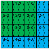
We have seen the DP algorithm that Floyd-Warshall deploys to compute APSP. Let us visualize to some extent as to how it is done for 4 vertices.

What Cells Are Used to Optimize

The computation will be done using k = 1 to 4, in the following order – starting with cell 1-1, 1-2, . . . . .2-1, 2-2, …….3-1, ……. 4-3, 4-4.

At first, using k = 1.

Let us see how the paths are improving using the following two examples.

dist[2][3] = min (dist[2][3],  dist[2][1] + dist[1][3])

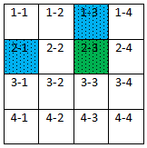
and dist[3][4] = min (dist[3][4],  dist[3][1] + dist[1][4])

We see that for k = 1, all paths are optimized using paths from 1^st (k^th) row and 1^st (k^th) column.

K^th Row and Column do not Change

What about paths on k^th row and k^th column?

dist[1][2] = min(dist[1][2], dist[1][1] + dist[1][2]) – well, there is no point in updating dist[1][2] by adding something more to it.

So we see, at a certain k^th iteration, k^th row and k^th column used to update the rest of the paths while they themselves are not changed.

At k = 1

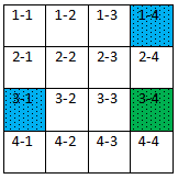
At k = 2

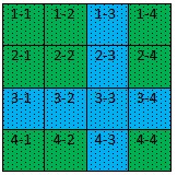
At k = 3

At k = 4

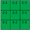
Consider Only 3X3 Matrix Was Computed

Now assume that we did not consider that we had 4 vertices. Rather we considered that we had 3 vertices and completed APSP computations for all paths in the 3X3 matrix. We ignored the 4^th row and column altogether.

So we have APSP computed for the following matrix using k = 1, 2 and 3.

Add 4^th Vertex

Let’s say, 4^th vertex arrives now. First, we can compare the computations used for the above 3X3 matrix with the same for the 4X4 matrix as shown earlier and find out what all computations need to be done now to extend this 3X3 matrix to 4X4 matrix to accommodate the new 4^th vertex.

We will find that at first we have to optimize the 4^th row and column using k = 1, 2 and 3. Let us do that.

Note that at this point, 4^th row and column are not used to optimize paths for the older 3X3 matrix. So now that we have the 4^th row and column optimized using k = 1, 2 and 3, we have to optimize that 3X3 matrix using k = 4.

This way, we don’t miss out any computation had we considered all the 4 vertices at one go. And thus we are done with optimizing all the paths in the 4X4 matrix.

Code

dist[][] //APSP matrix, already computed for n-1 vertices

p[][] //predecessor matrix, already computed for n-1 vertices


dist[n][] = ∞

dist[][n] = ∞

dist[n][n] = 0


for each edge (i, n)

  dist[i][n] = weight(i, n)

  p[i][n] = n


for each edge (n, i)

  dist[n][i] = weight(n, i)

  p[n][i] = i


for k = 1 to n-1

  for i = 1 to n-1

    if dist[i][n] > dist[i][k] + dist[k][n]

      dist[i][n] = dist[i][k] + dist[k][n]

      p[i][n] = p[i][k]

  for j = 1 to n

    if dist[n][j] > dist[n][k] + dist[k][j]

      dist[n][j] = dist[n][k] + dist[k][j]

      p[n][j] = p[n][k]


for i = 1 to n-1

    for j = 1 to n-1

      if dist[i][j] > dist[i][n] + dist[n][j]

        dist[i][j] = dist[i][n] + dist[n][j]

        p[i][j] = p[i][n]

Complexity

The complexity for this incremental building for a new vertex is clearly O(n²). That makes sense. After all, for n vertices the cost is O(n³) that is the cost of Floyd-Warshall, had all n vertices were considered at one go.

But this incremental building makes a huge difference. For example, consider that we have 1000 vertices for which we have already computed APSP using 1 billion computations. Now that 1001^st vertex arrives, we can accommodate the new vertex with a cost of 1 million (approx.) computations instead of doing 1 billion+ computations again from the scratch – something that can be infeasible for many applications.

Printing Arbitrage Path

We can find the first negative cycle by looking (for a negative value) at the diagonals of the dist[][] matrix, if exists and then print the associated path. For path reconstruction, we can follow the steps as described here.

GitHub: Code will be updated in a week

Index