Pranjal’s ML algorithm wins him a Silver Award at SSEF 2025.
It is quite interesting that young secondary / high school students are introduced to research, a field traditionally reserved for PhD students and seasoned researchers. Around 350 finalist research works and projects in various scientific domains at SSEF 2025 is a good testament that students are responding to this very well.
My sincere thanks to all organisers and educators and wishing all the best to all participants.
Category: Machine Learning
Models in Machine Learning
15th Friday Fun Session (Part 1) – 28th Apr 2017
Usually, machine learning algorithms build a model. We are trying to understand what a model looks like and some associated concepts around it.
Descriptive vs. predictive analytics
Descriptive analytics looks at historical data to understand what happened. It describes historical data using different statistical techniques and visualization.
Predictive analytics looks at historical data to understand and predict future. It also uses different statistical techniques, machine learning algorithms etc.
Both can have models, called as descriptive and predictive models. Here by model we are referring to predictive model.
Understanding model
The globe of the Earth does not show every detail of it but this small model can be put on our desk and it can give us an idea as to how the Earth looks like. When we talk about machine learning model, it is similar to that. It represents the data that is used to build it.
Suppose we have some employee data as shown in the table below.

We want to build a model using this data set. Later, given an employee’s salary and experience, we would like to know her designation, using it.
Model as logical statement or rule
Based on the above data, we can construct two logical statements as shown below.
If salary is more than 3,000 and experience is more than 5 years
then the employee is a Senior Software Engineer.

Otherwise, the employee is a Junior Software Engineer
Given an employee’s salary and experience, we can find her designation by using the above formula. That formula is called the model.
Model as function
The formula can take the form of a function as well. Let us draw a function that can work as a model for the above data set.
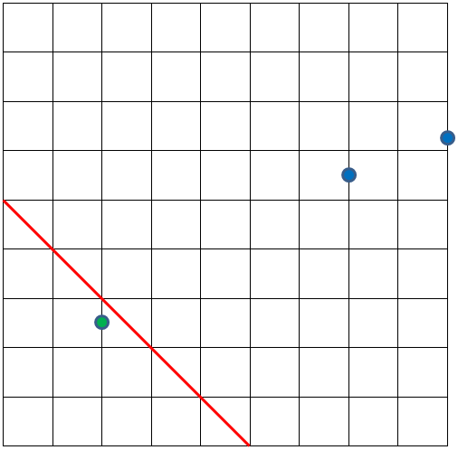
We have used X-axis for experience, and Y-axis for salary (in thousands). The three data points would be placed as shown above.
The red line can work as a model. All employees on the left side of it, shown as green points are Junior Software Engineers. And all employees on the right side of it, shown as blue points, are Senior Software Engineers.
Note that, this model is not an exact translation/equivalent of the earlier model expressed as logical statements. Meaning, the same input data might be classified (Junior Software Engineer or Senior Software Engineer) differently.
The (red) line equation can be written as
   x + y = 5
=> x + y - 5 = 0
=> f(x, y) = x + y - 5

The model can be expressed this way:
if f(x,y) >= 0, then Senior Software Engineer
if f(x,y) < 0, then Junior Software Engineer
If a new employee input comes with salary 4,500, and experience 1 year, this model would classify her as a Senior Software Engineer.
   f(x, y) = x + y - 5
=> f(x,y) = 4.5 + 1 - 5
=> f(x,y) = 0.5
=> f(x, y) >= 0
If we use the earlier model to classify this input, it would classify it as Junior Software Engineer – different prediction!
Hybrid model
A model can use a combination of both logical statement and function.
To summarize, a model can be expressed using logical statement, function or a hybrid of both.
When a model is built?
At the beginning when we have some data, usually we split it into training data and test data; we provide the training data to a machine learning algorithm that in turn builds a model. Then we use the test data to check how this model is performing and tune the model, as and if required. The model can be further updated, say, periodically, when more data is gathered.
Different machine learning algorithms build different kinds of model. Some build at first, some delay it.
Eager vs. Lazy learning
When a machine learning algorithm builds a model soon after receiving training data set, it is called eager learning. It is called eager; because, when it gets the data set, the first thing it does – build the model. Then it forgets the training data. Later, when an input data comes, it uses this model to evaluate it. Most machine learning algorithms are eager learners.
On the contrary, when a machine learning algorithm does not build a model immediately after receiving the training data, rather waits till it is provided with an input data to evaluate, it is called lazy learning. It is called lazy; because, it delays building a model, if it builds any, until it is absolutely necessary. When it gets training data, it only stores them. Later, when input data comes, only then it uses this stored data to evaluate the result.
There is a different set of pros and cons associated with eager and lazy learning. It is obvious that lazy learning would take less time during training but more time during prediction.
Eager learning builds a model for the whole data set, meaning it generalizes the data set, at the beginning. It might suffer accuracy compare to lazy learning that has more options in terms of the availability of the whole data set as well as the mechanisms to make use of it.
Lazy learning is typically divided into two types: instance-based learning and lazy Bayesian rules.
Instance-based learning
Do all machine learning algorithms build a model?
No, all machine learning algorithms don’t build a model, when by model we mean generalizing the data. For example, decision tree builds a model but k-NN does not.
A row is also called an instance, meaning a set of attributes. Hence a set of training data is also called a set of instances. When a machine learning algorithm does not build a model, rather uses the set of instances directly to evaluate the result, it is called instance-based learning. It is also called memory based learning as it memorizes the whole data set. For the same reason it is also called rote learning.
Instance-based learning, as mentioned above is one kind of lazy learning.
Supervised, unsupervised and semi-supervised learning
The employee example that we have discussed here is an example of supervised learning. Here we wanted to predict an output variable – designation of an employee by providing input variables – salary and experience. While building the model, we provided training data having most (all for the example here) values for input variables and all values for the corresponding output variable.
An important requirement of supervised learning is that, for all the training data we must provide the output variable value. Because, supervised learning learns from it. Most machine learning algorithms use supervised learning.
However, some machine learning algorithms don’t predict an output variable. They just take only the input variables and try to understand, say the distribution or pattern of the data. They are classified mainly into clustering and association rules. For example, when we do clustering, it might come up and say the given data falls into 3 groups.
There is a third type of learning, in the middle of supervised and unsupervised, called semi-supervised. In many real life examples, a good portion of the training data does not have labels for the target variable, meaning many instances of the training data don’t have the output attribute value known. It might be expensive to label them as it might require domain experts.
In this situation, unsupervised learning comes to rescue. It labels them, and then the labelled data is fed into supervised algorithm (to build model) for prediction. This process (unsupervised algorithm labels them and supervised algorithm predicts), might be repeated unless satisfactory accuracy is acquired.
In the above example, we have seen examples of supervised models. However, predictive models include unsupervised and semi-supervised models as well, the latter being a combination of supervised and unsupervised models.
Parametric vs. non-parametric model
Some machine learning algorithms would come up with a model with a predetermined form. For example, it would construct a function with 2 parameters. Now given the training set it would compute that two parameters and come up with a function. An example would be naive Bayes. They are called parametric. For prediction they would depend on this function alone.
On the other hand, some machine learning algorithms would construct a model based on the information derived from the data. For example, k-NN, C4.5 – a decision tree etc. They are called non-parametric. Non-parametric does not mean no parameter, rather no predetermined parameters.
k-NN as an example of a non-parametric model might create a little confusion as k-NN does not build any model at the first place. Well, here model is used in a broader sense to mean how it computes output value. K-NN uses the complete training data set to do so. Hence the whole training data set is the input parameter. Adding one more training data can be thought as increasing the parameter by one. That perfectly matches another definition of non-parametric model that says – the number of parameters grows with the amount of training data.
Classification vs. regression
The model that we are discussing so far – given salary and experience, predict the designation, is called a classification model. The reason is the output variable, designation – a categorical variable. Meaning, it would take one of the predefined categories or classes. In this example, there are two categories or classes: Junior Software Engineer and Senior Software Engineer.
Let us alter the input and output a bit for the model. Suppose the model would now predict the salary, given experience and designation. Then this model would be called a regression model. The reason is the output variable, salary – a continuous variable. Meaning, it can take any value, not limited by a predefined set of classes, unlike earlier example.
Bias vs. variance
Let us continue with the previous example of the model that predicts salary. Ideally, the salary would be calculated by taking the input values, experience and designation into consideration.
But assume the model that is built by a machine learning algorithm, is so simple and dumb. Let us say, given the training data, it computes the average of the salary (2500 + 5500 + 6200) / 3 = 4733 by ignoring all other parameters. Now when an input comes asking the salary, it does not care the experience or designation of the input. The only output (salary) that comes out of it is 4733. Now that is called a highly biased model. It generalizes the data so much that it ignores the input values of the training data and hence underfits the training data. A biased model that does not distinguish a 2 years experienced Junior Software Engineer from a 15 years experienced Senior Software Engineer, and predicts the same salary of 4733 for both, is not a good model, for obvious reasons.
By the way, what machine learning algorithm can possibly come up with such a model and under what condition?
On the other extreme, there is this model with high variance that considers each minute detail of the training data that is possibly nothing but noise, to be the ultimate truth and incorporates them into the model. Hence it is said to be overfitting the training data, and results in a highly complex model. However, a model with all these intricate truths of training data, even though performs very well with training data (after all, the model is built to overfit the training data), do not stand the test of real world. This kind of model, with highly fluctuating prediction, due to little changes in input parameters, is not desirable either.
What we need is a balance, a trade-off between bias and variance; achieving which is a prerequisite, for a good model.
Maximum Subarray Problem
21st Friday Fun Session – 9th Jun 2017
Maximum subarray finds the contiguous subarray within a one-dimensional array having the largest sum.
Visualizing the divide and conquer solution
For the time being, let us forget about maximum subarray problem and focus on the divide and conquer solution that we discussed in the previous session.
If we visualize the tree, we see that from the left subtree the smallest value is propagated upwards. On the way up, it is treated as the buy value and the right side values are treated as sell values. This way profits are calculated and maximum among them is retained. So we see two themes of processing as we go from left to right of the array:
- Retain the minimum value and treat it as the buy value.
- Calculate profit by treating each value seen as we go right and retain the maximum profit.

The above table shows day number in first row and the corresponding stock prices in second row. Third row shows the minimum value seen so far. The fourth row shows the profit had we sold on this day, buy price being the minimum value seen so far (shown in green).
The intuition
The intuition being, when we see a new lower value than the one already seen, we treat that as the new buy value. For example, when we see the new lower value 1 on day 5, onward we treat that as the new buy value and calculate profits considering each of the following days as sell days. This is because the new lower value (lowest till now) would give a better profit when the following days are treated as potential sell days. By treating the previous lower value 2 that was found on day 1, we already considered all possible profits prior to 5th day and retained the best among them. On 5th day, the utility of the previous lower value, which is 2, stops.
From divide and conquer to dynamic programming
Now let us now consider the dynamic programming (DP) point of view. In dynamic programming we make use of the result of an already solved overlapping subproblem.
On the first day, we can buy but cannot sell. After all, no profit would be made selling on the first day with the same price as the buy price. Also note that we have to buy and only then we can sell. So on day 1, profit is 0. Now if we want to find the best profit on day 2, can we use the solution of the previously solved overlapping subproblem? What is that already solved overlapping subproblem at day 2? Well, it is the best profit found for day 1, which is 0. How can we make use of the previous solution to find the best profit at day 2? Well, we have to consider two things:
- If we have to make the most profit by selling today, then we have to buy using the lowest price seen so far.
- If the profit calculated above is better than the best seen on previous day, then this is the new best. Else previous day’s best is still the best for today.
For example, on day 2 we realize that we can make a profit of (8-0) = 8 and it is better than the profit at day 1, which is 0. Hence, the best profit for day 2 is updated to 8. On day 3, we find we can make a profit of 3 but the best profit till day 2 is better than this. So, we retain day 2’s best profit as day 3 best profit.
So we realize, what we found by visualizing and transforming the divide and conquer solution is nothing but this dynamic programming. In fact, this is possibly one of the simplest forms of dynamic programming.
The below code would find the solution. For brevity buy day and sell day is not tracked that is easy to accommodate.
void StockDpN(double price[], int n, double &maxProfit)
{
  double minPriceSoFar = price[0];
  maxProfit = 0;

  for(int i=1; i<n; i++)
  {
    if(price[i] - minPriceSoFar > maxProfit)
      maxProfit = price[i] - minPriceSoFar;

    if(price[i] < minPriceSoFar)
     minPriceSoFar = price[i];
  }
}
The reverse can also be used. If we start from right and move leftwards, we have to keep track of the maximum value seen so far and that is the sell value. As we go left, we see new values and they are buy values. The associated code is not shown here.
Moving to maximum subarray problem
Suppose we buy a stock at one day and then sell it on the following day. For example, buy at day 1 and then sell on day 2. Buy at day 2 and then sell on day 3 and so on. Each day we make a profit, incur a loss and sometimes it is neutral, meaning no profit or loss (buy value and sell value being the same). The third row of the below table shows the same (loss shown in red).

The optimal solution to our stock profit problem with our example set is to buy on day 1 at price 2 and sell it on day 4 at price 12, thus making a profit of 10. It is the same as saying:
- We buy at day 1 and sell at day 2 making profit 8 and then
- Buy at day 2 and sell at day 3 making loss 5 and then
- Buy at 3 and sell at day 4 making profit 7 and then
- Add all profits/losses made in our buy/sell operations that started by buying on day 1 and ended by selling on day 4. The final and best profit is: 8 + (-5) + 7 = 10.
Thus we have transformed the previous stock profit problem to a maximum subarray problem. As explained earlier, we are interested to find contiguous portion of array that gives the maximum sum. In the above 8 values that we have, we got two such subarrays each giving a sum of 10. They are showed in colored boxes.
Kadane’s algorithm
Kadane’s algorithm also deploys DP to solve this. Once again in DP, we have to make use of already solved overlapping subproblems. Here it is done by this way:
- Maximum subarray ending in position i+1 includes already solved maximum subarray ending at i, if doing so increases the sum for subarray ending at i+1
- Else maximum subarray ending in position i+1 will only have itself.

Maximum subarray at day 1: day 1 value which is 0.
Maximum subarray at day 2: since adding the subarray sum for day 1, which is 0, is not increasing the sum for day 2, maximum subarray at day 2 will have only day 2 value itself, meaning 8.
Maximum subarray at day 3: subarray sum at day 2 is positive, which is 8, and helping day 3, so subarray at day 3 includes day 2. Subarray sum at day 3 = 8 + (-5) = 3.
It boils down to a simple thing. If the previous sum is positive then take it forward else not. The red color in the Maximum subarray sum row (4th row) shows the cases where it does not include the (immediately) prior subarray. In two cases it happens (8 at day 2 and 2 at day 6) because the prior sums (0 and -1 respectively) are not more than zero.
The code shown below implements this. Note that the input array profit contains the profit and loss unlike the earlier DP function where we passed the stock prices. It is also noteworthy that if all values are positive then the whole array is the maximum subarray. After all, adding all of them would give the highest sum.
void StockKadaneDpN(double profit[], int n, double &maxProfit)
{
  double curProfit = 0; maxProfit = 0;

  for(int i=1; i<n; i++)
  {
    curProfit = curProfit > 0 ? curProfit + profit[i] : profit[i];
    if(curProfit > maxProfit)
      maxProfit = curProfit;
  }
}
If we observe closely, we see that this DP is essentially the same as the one we discussed earlier in this post.
Backtrace
At the end, when we find the maximum subarray sum 10 at day 4, we will do what is called backtrace, typical of DP to find the path, in this case, the maximum subarray. We know that at day 4, we included the subarray ending at day 3. At day 3, we included the subarray ending at day 2. At day 2, we did not include prior subarray. So the maximum subarray starts at day 2 and ends at day 4. It could be easily tracked/stored as we went ahead in the computation using appropriate data structure and would not require a come back.
Map maximum subarray solution to stock profit
If we want to map this solution back to our stock profit problem, then we know the profit at start day of the maximum subarray, that is day 2, is essentially found by buying stock at the previous day that is day 1. So the solution is: buy at day 1 and sell at the last day of the maximum subarray that is day 4. And the profit would be the maximum subarray sum that is 10.
The transformations
This is an interesting problem to observe as we started with a O(n^2) brute force accumulator pattern, moved to O(n log n) divide and conquer that we optimized later to O(n). Finally, we transformed that to a O(n) DP solution only to find that it is interchangeable to O(n) maximum subarray problem that is also a DP solution.
Can we do better than O(n)? Well, that is not possible. After all, we cannot decide the best solution unless we read all the data at least once. Reading the data once is already O(n).
Where is pattern recognition here?
Maximum subarray essentially gives the brightest spot in a one-dimensional array. Finding this brightest spot is one kind of pattern recognition. Note that we just solved a problem that reads like this: given the profit/ loss made by a company over the period find the longest duration(s) when the company performed the best. The answer here is: from day 2 to day 4 or from day 6 to day 7.
Even though we focused on finding the single brightest spot, it is also possible to find, k brightest spots.
Again, maximum subarray considers only one dimension. In real life, data sets typically contain more than one dimension. For example, a problem involving two dimensions might read like: can you find the largest segment of the customers buying product x based on age and income? A potential answer might be: customer from age 30 to 40 years with income range $3000 – $6000. There are other algorithms to deal with multi-dimensional data.
GitHub: Stock Profit Kadane Code
k-d Tree and Nearest Neighbor Search
18th Friday Fun Session – 19th May 2017
We use k-d tree, shortened form of k-dimensional tree, to store data efficiently so that range query, nearest neighbor search (NN) etc. can be done efficiently.
What is k-dimensional data?
If we have a set of ages say, {20, 45, 36, 75, 87, 69, 18}, these are one dimensional data. Because each data in the array is a single value that represents age.
What if instead of only age we have to also store the salary for a person? The data would look like [{20, 1500}, {45, 5000}, {36, 4000}, {75, 2000}, {87, 0}, {18, 1000}]. This data is two dimensional as each data set contains two values. Similarly, if we add one more attribute to it, say education it would be a 3 dimensional data and so on.
Why are we talking about efficiency?
Suppose, given a data point {43, 4650}, we want to know which person has a similar profile. In this particular example, it would be {45, 5000} whose age and salary both are close to this input. If we want the second closest person, it would be {36, 4000}. How did we find that? Well, we could iterate over the 6 data points and check against each of them. We would end up doing comparison against each of them. That is O(n) complexity. Not bad, but when we have millions of points it would be very expensive.
When we have just one dimension, instead of a linear search with O(n) complexity, we use Binary Search Tree (BST) with O(log2(n)) complexity. The difference is huge. For a million rows where linear search would take one million comparisons, binary search would take only 20 comparisons. This is because O(n) = O(1000, 000), meaning 1000, 000 comparisons and O(log2(n)) = O(log2(1000, 000)), meaning 20 comparisons. If each operation takes 1 millisecond BST would take 20 milliseconds, whereas linear search would take 1000 sec, almost 16 minutes. 20 milliseconds vs. 16 minutes.
How do we split the points?
We can extend BST to do this. This is what Jon Louis Bentley created in 1975. K-d tree is called 2-d tree or k-d tree with 2-dimension when k = 2 and so on. In BST, at each level of the tree we split the data points based on the data value. Since, BST deals with just one dimension the question does not arise which dimension. But in k-d tree since we have more than one dimension. At each level we can choose to split the data based on only one dimension. So if we have 3 dimensions: x, y and z, at first level we split the data sets using x dimension. At 2nd level we do so using y dimension and at 3rd level we use z dimension. At 4th level we start again with x dimension and so on. Of course, we can continue splitting only if we have more data left. If we are splitting the points based on x dimension for a certain level then we call x the cutting dimension for this level.

Where do the data points reside?
A k-d tree can have all the data points residing only in the leaf nodes. The intermediary nodes could be used to save the (non-data) splitting values. Alternatively, all nodes – internal and leaf, could save data points. In our case, we are saving data in all nodes.
Balanced or Skewed
The above tree looks very symmetrical. That means, both the left sub-tree of right sub-tree having almost the same number of nodes. If the height of left and right sub-tree differs at max by 1 then it is called a balanced tree.
The more a tree is balanced the more efficient it is to do search and other operations on it. For example, if we have to do a search for a number in the above tree with height = 3, it would take at max 4 (height + 1) probes. If it were a skewed tree where most or all nodes reside on the same side, it would have taken 15 probes in the worst case, similar to a linear search.
How can we build a balanced tree?
Let us start with an example set to walk through for the rest of the post. Say, we have 13 points in a two dimensional space. They are: (1, 3), (1, 8), (2, 2), (2, 10), (3, 6), (4, 1), (5, 4), (6, 8), (7, 4), (7, 7), (8, 2), (8, 5) and (9, 9) respectively.
Say, at level 1 the first dimension, say x is chosen as the cutting dimension. Since we want half the points to fall on the left side and the rest half on the right side we can simply sort (typically with O(n log2(n)) complexity) he data points on x dimension and chose the middle as the root. We make sure that we remain consistent in choosing for left side points whose cutting dimension value is less than the same for root and more than or equal to for the right.
In this example, if we sort the 13 points based on the x dimension values then the root would be (5, 4). So with (5, 4) being the root at level 1, the left side points would be: (1, 3), (1, 8), (2, 2), (2, 10), (3, 6), and (4, 1). And the right side points would be (6, 8), (7, 4), (7, 7), (8, 2), (8, 5) and (9, 9). We call the tree building procedure recursively for each half data sets. We also indicate that y dimension of the data point would be chosen as the cutting dimension for the next level sub-trees.
Now we have the following data points to build the left side tree with cutting dimension being y: (1, 3), (1, 8), (2, 2), (2, 10), (3, 6), and (4, 1). We can chose (3, 6) as the root, at level 2 after sorting them according to y dimension. The left side points would be (4, 1), (2, 2), and (1, 3) and the right side points would be (1, 8) and (2, 10).
At the end the tree would look like below:

Bounding Box
We could visualize the points and the tree it in a different way. Let us put the 2 dimensional 13 points in x-y coordinate system.
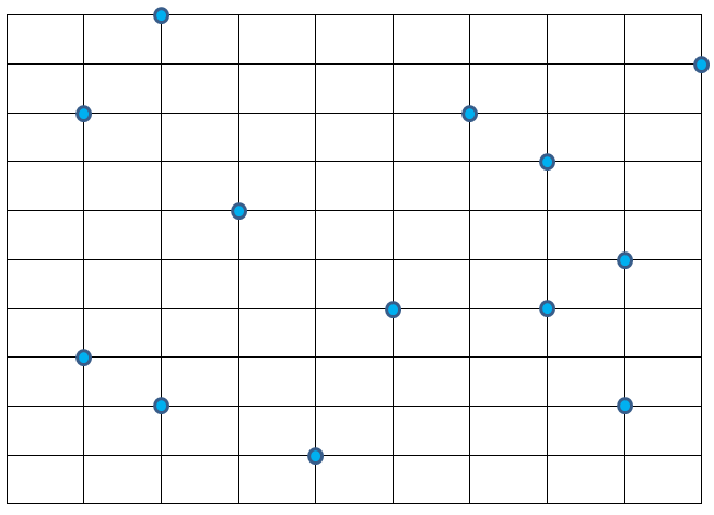
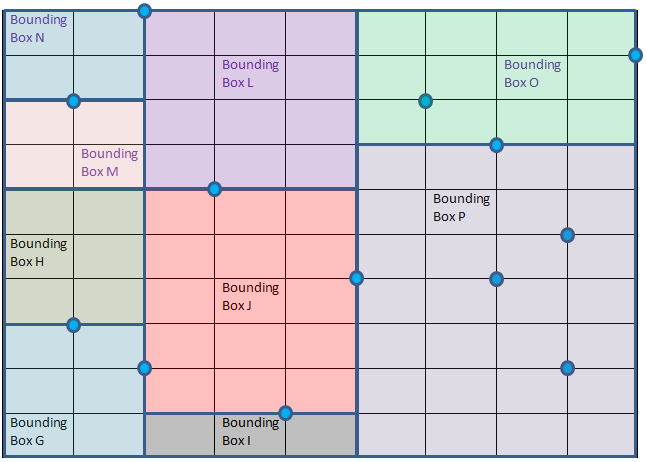
The root (5, 4) at level 1 owns the whole bounding box. This root then divides the whole region into two bounding boxes: bounding box A and bounding box B, owned by second level roots (3, 6) and (8, 2) respectively.

Root (3, 6) would then divide the bounding box A into bounding box C and D owned by 3rd level roots (2, 2) and (2, 10) respectively. It does so using y as the cutting dimension meaning splitting the points inside A based on y dimension values.
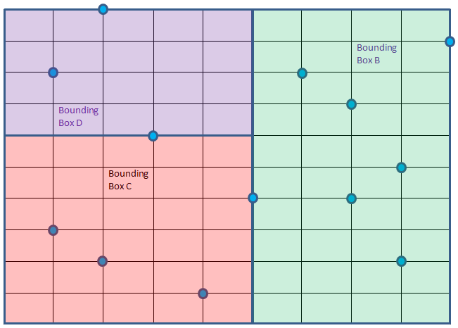
Bounding box C rooted at (2, 2) is further divided into E and F, this time using x as the cutting dimension.
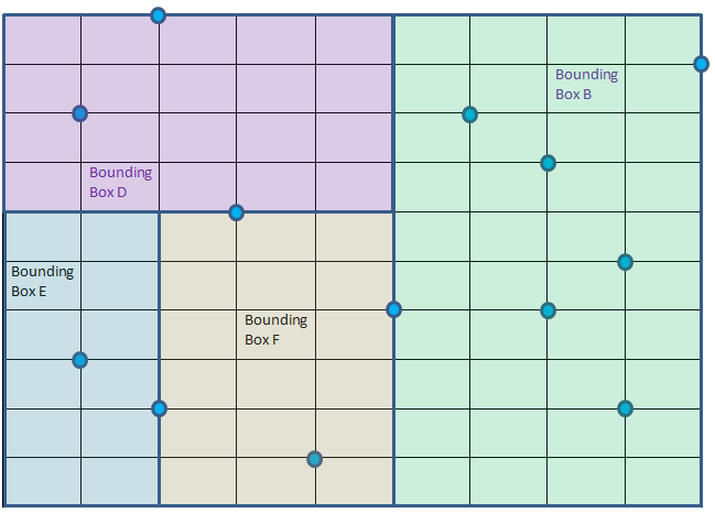
Bounding box E can be further divided into G and H using cutting dimension y but none of them has any point. Similarly, bounding box F can be further divided into I and J using cutting dimension y, once again none of them has any point.
Bounding box D can be divided into K and L using cutting dimension x. K having one point while L having no point inside it. K is further divided into two M and N using cutting dimension y having no points left for any of them.
Similarly bounding box B will be divided into smaller boxes.
The final bounding boxes are shown below. Even though bigger bounding boxes like A is not shown here, they are all present nonetheless. Only first level division of the B bounding box is shown where (7, 7) has split it into O and P.
Nearest Neighbor Search
How many neighbors do we want?
We are interested to get k nearest neighbors, where k can be 1 2, 3 or any value. However, we will first see how to get the closest one point. It can then be easily extended to understand how to get more.
Points inside the same box of the query point are not necessarily the closest to query point
Suppose, we have to find the nearest neighbor of Query point Q = (4, 8) as shown below in red color. It falls inside bounding box D. But it is obvious that the closest point to Q does not fall within box D, rather it is inside Box B. Well, you can see point (6, 8) is the closest to Q. A person living near the Western border of Singapore is closer to a person living in the adjacent border of Malaysia than a person living in the eastern side of Singapore.
How to find the closest point?
We will extend the same binary search principle here. We start at root and then traverse down the tree finding the promising bounding boxes to search first and at the same time skip bounding boxes where the chance to get a closer point than the closest one to the query point found so far are thinner.
We will maintain the closest point (to Q) and minimum distance (distance between closest point and Q) found so far, at first they are null and infinite respectively. We start at root, with cutting dimension being x and do the following:
- If we reach a null node return.
- If the boundary box owned by the present root has no chance of having a point closer than minimum distance then return, meaning skip traversing that sub-tree altogether. We do so by checking the distance from Q to the bounding box. In two dimension case, it is Q to a rectangle (not a distance from Q to an actual point in the bounding box). This is how we prune search space.
- If the present root is closer to Q than minimum distance, we save it as the closest point and also update the minimum distance.
- Now we have two choices: traverse left sub-tree or traverse right sub-tree. We will compare the cutting dimension (at level 1 it is x, at level 2 it is y, at level 3 it is again x and so on) value of Q to that of root. If Q’s x is dimension value is smaller than that of root then we traverse left first, right second. So we are calling both of them but at a certain order with the hope that the first traversed sub-tree would give a closer point than any point the other side sub-tree could possibly offer. So next time when we would traverse the other sub-tree we can do a quick check and completely skip traversing that sub-tree. Something that might not materialize as well.
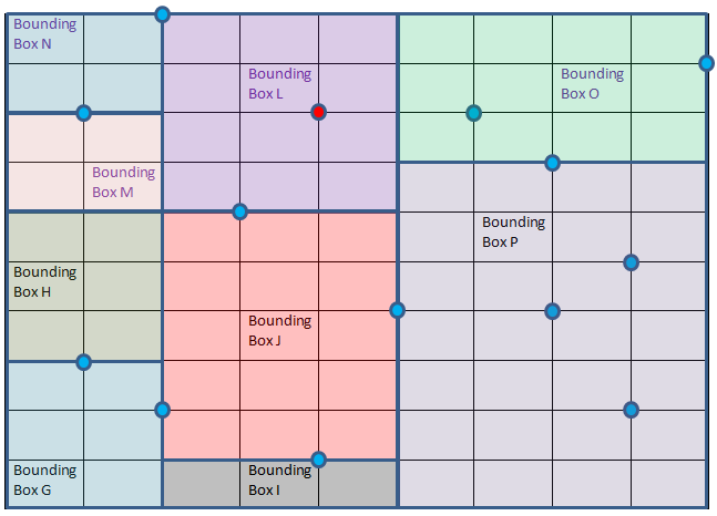
Let us walk through this particular example. At root (5, 4), closest point so far is null, minimum distance is also null. We set the root as the closet point and minimum distance (using commonly used Euclidean distance for continuous values) to ((x1 – x2)2 + (y1 –y2)2)1/2 = 4.12 (approx.). Now we have two bounding boxes A and B. The decision that we need to make is which one to traverse first? Q’s x dimension value 4 is smaller than root’s x dimension value that is 5. So we choose left first, right second. Both of them are to be called by using the cutting dimension y. The bounding box for each of the call is going to change. Well, we know each root owns a bounding box.
At the second call, root is (3, 6), bounding box is A. Distance from Q to A is zero as Q is within A. So we cannot skip traversing this sub-tree. Distance from (3, 6) to Q (4, 8) is 2.24, closer than existing minimum distance 4.12. Hence, we update our closest point to (3, 6) and minimum distance to 2.24. Next decision to make is again which side to traverse first. We have Q’s y value 8 that is more than present root’s y value 6. So we will traverse the right side first, left side second.
Next, the function is called with root, (2, 10), cutting dimension x and bounding box D. Distance between (2, 10) and Q (4, 8) = 2.83 that is larger than existing minimum distance. So we are not updating the closest point in this call. Next – choose which side to traverse first. Q’s x dimension 4 is bigger than root’s x dimension 2, hence right sub-tree is chosen first that is null anyway. So the call to it will return without doing anything.
Next call would be made with root (1, 8) that is 3 units away from Q. No improvement for the closest point. Also this root has no children. We have reached bottom of this side of the tree in our DFS search.
Next call is done with root (2, 2), far away from Q. But the bounding box owned by it is only 2 units away from Q. Hence, there is a chance that we might end up getting a closer point from this area. Hence, we cannot skip this tree. Right side to traverse first based on x dimension value comparison.
Root (4, 1), that is 8 units away from Q is called. It owns bounding box F that is 2 units away from Q. Once again cannot skip this area. Well, it has no child anyway.
Root (1, 3) is called that owns bounding box E that is 2.83 units away from Q, having no chance to offer any closer point. For the first time we can skip this area/sub-tree/bounding box.
We are done with the left side of level 1 root (5, 4). Now traverse right side.
Sub-tree with root (7, 7) owing bounding box O is called. Subsequently sub-tree rooted at (6, 8) would be called and that would be the closest point at distance 2.
How much search space did we prune?
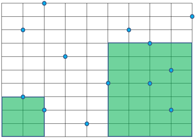
We will skip traversing the left sub-tree rooted at (8, 2) that owns bounding box P. In terms of nodes we skipped only 4 nodes, 3 of them are rooted at (8, 2). Previously we skipped sub-tree rooted at (1, 3) as well. The green areas were pruned, meaning we did not search there. That was not quite efficient though!
How to get k nearest neighbors?
Instead of keeping a single closest point we could maintain a priority queue (max heap) to keep k (say 2, 3 or any number) closest points. The first k points would be en-queued anyway. Onwards, a new point, if better, would replace the worst of the closest point found so far. That way we can maintain the k nearest points easily.
Too few points is a problem
If we have to construct a k-d tree with 20 dimensional data sets, we got to have around 220 data points. If we don’t have enough data then at many levels we will not have sufficient data to split. We will also end up with an unbalanced k-d tree where search and other operations would not be very efficient.
In general, we need k-d tree when we have higher dimensional data points. But when the dimension is too high other approaches might work better.

