Executing SP using EF

34th Friday Fun Session (Part 1) – 22nd Sep 2017

Many a times, we use Entity Framework (EF), Microsoft’s recommended data access technology for an application, to execute (MS SQL Server) Stored Procedure (SP), and retrieve the results emitted by them. Here we discuss different kinds of output that a SP can produce and how we can retrieve them using EF.

SP output

A SP typically provides the following kinds of results:

  1. Return code (single integer)
  2. Output parameters (one or more, any data type)
  3. Result set
    1. Single result set
    2. Multiple result set
      1. All having the same schema
      2. Having different schema

Return code

SP can return a single integer return code. Return statement without any value (null) would automatically return 0. It is mostly used to exit execution of a SP when certain condition is met.

CREATE Procedure SpReturnCode
AS
BEGIN
  RETURN 1;
END

Using T-SQL we can execute SP like below.

DECLARE @Success AS INT
EXEC @Success = [SpReturnCode];
PRINT @Success

Output parameter

SP can return one or more values, each having its own data type.

CREATE Procedure SpOutputParameter (@InputValue INT, @OutputValue INT OUTPUT)
AS
BEGIN
  SET @OutputValue = @InputValue + 1;
  RETURN 0;
END

Using T-SQL we can execute SP like below.

DECLARE @ReturnValue INT;
EXECUTE [SpOutputParameter] 2, @ReturnValue OUTPUT;
PRINT @ReturnValue

Single result set

Returns a result set having 0 or more rows of a certain schema. The following SP returns a result set with a single column named, Success.

CREATE Procedure SpSingleResultSet
AS
BEGIN
  SELECT 3 AS Success
  RETURN 0;
END

Multiple result set, same schema

The following SP returns the result set for Employee schema twice.

CREATE Procedure SpMultipleResultSetSameSchema
AS
BEGIN
  SELECT * FROM [Employee]
  SELECT * FROM [Employee] SELECT [EmployeeId] > 10

  RETURN 0;
END

The following SP returns a result set that is not associated with any database entity.

CREATE Procedure SpMultipleResultSetNonDbContextEntity
AS
BEGIN
  DECLARE @Loop AS INT
  SET @Loop = 0

  WHILE @Loop < 10
  BEGIN
    EXEC SpSingleResultSet
    SET @Loop = @Loop + 1
  END

  RETURN 0;
END

Multiple result set, multiple schema

The following SP returns two different result sets: one for Company and another for Employee.

CREATE Procedure SpMultipleResultSetMultipleSchema
AS
BEGIN
  SELECT * FROM [Company]
  SELECT * FROM [Employee]

  RETURN 0;
END

Executing SP using EF

We will use the following different ways in EF to read different kinds of SP output as described earlier:

  1. ExecuteSqlCommand
  2. SqlQuery
  3. CreateCommand/ExecuteReader

ExecuteSqlCommand

This executes a given DDL/DML command. This can be executed when no result set needs to be returned.

Return code

Return code does not require any explicit output parameter to be used in the SP. However, while calling from EF, it should be treated as an output parameter by specifying the direction for the parameter.

SqlParameter returnCode = new SqlParameter("@ReturnCode", SqlDbType.Int);
returnCode.Direction = ParameterDirection.Output;

Db.Database.ExecuteSqlCommand("exec @ReturnCode = [SpReturnCode] ", returnCode);
var returnCodeValue = (int)returnCode.Value;

Output Parameter

For each of the output parameters, we need to declare an output parameter in EF matching the appropriate data type.

SqlParameter inputParam = new SqlParameter("@InputValue", SqlDbType.Int);
inputParam.Direction = ParameterDirection.Input;

SqlParameter outputParam = new SqlParameter("@OutputValue ", SqlDbType.Int);
outputParam.Direction = ParameterDirection.Output;

Db.Database.ExecuteSqlCommand("[SpOutputParameter] @InputValue, @OutputValue OUT", inputParam, outputParam);
var returnValue = (int)outputParam.Value;

SqlQuery

SqlQuery is usually used when SP returns a single result set. However, it can return any data type including primitive types – not necessarily only entity type. If the SP returns multiple result sets, it will only get the first one. However, the complete execution of the entire SP does happen.

public class SuccessSet
{
  public int Success { get; set; }
}

var result = Db.Database.SqlQuery("[SpSingleResultSet]").ToList();

CreateCommand/ExecuteReader

When multiple result sets to be returned this method can be used. We need to use IObjectContextAdapter interface that makes use explicit interface implementation.

Db.Database.Initialize(force: false);
var cmd = Db.Database.Connection.CreateCommand();
cmd.CommandText = "[SpMultipleResultSetSameSchema]";

Db.Database.Connection.Open();

var reader = cmd.ExecuteReader();
var employees =
  ((System.Data.Entity.Infrastructure.IObjectContextAdapter)Db)
    .ObjectContext
    .Translate<Employee>(reader, "Employee", System.Data.Entity.Core.Objects.MergeOption.AppendOnly);

foreach (var employee in employees)
  Console.WriteLine(employee. Name);

While(!reader.NextResult())
{
  employees =
    ((System.Data.Entity.Infrastructure.IObjectContextAdapter)Db)
    .ObjectContext
    .Translate<Employee>(reader, "Employee", System.Data.Entity.Core.Objects.MergeOption.AppendOnly);

  foreach (var employee in employees)
    Console.WriteLine(employee. Name);
}

Db.GetDatabase().Connection.Close();

When result set is not in DbContext, slight modification is required.

var successSets =
  ((System.Data.Entity.Infrastructure.IObjectContextAdapter)Db)
  .ObjectContext
  .Translate<SuccessSet>(reader);

When different schema are used we can still use the same, we just need to use the right object while translating.

var companies =
  ((System.Data.Entity.Infrastructure.IObjectContextAdapter)Db)
  .ObjectContext
  .Translate<Company>(reader, "Company", System.Data.Entity.Core.Objects.MergeOption.AppendOnly);

reader.NextResult();

var employees =
  ((System.Data.Entity.Infrastructure.IObjectContextAdapter)Db)
  .ObjectContext
  .Translate<Employee>(reader, "Employee", System.Data.Entity.Core.Objects.MergeOption.AppendOnly);

Index

Pseudo-polynomial Complexity

33rd Friday Fun Session (Part 2) – 15th Sep 2017

The complexity for FaaS solution is O(n), where n is the largest day number. It looks like polynomial. However, it is actually pseudo-polynomial.

Size of input

Complexity is measured in terms of the size of input, say, in bits. Suppose, there are b bits in n. Then O(n) = O(2b) and hence, it is exponential.

Let’s assume n increases from 10 to 1125899906842624. More specifically, lunch schedule, as used in the previous example, changes from 1, 3, 4, 5, 6, 7, 10 to 1, 3, 4, 5, 6, 7, 1125899906842624. We still have the same 7 days to go for lunch. Yet, we are running 1,125,899,906,842,624 loops. In our layman understanding, the problem is still the same and should have taken the same amount of time to execute, and yet, for the latter, the algorithm takes way too long!

Spot a pseudo-polynomial

This is how we spot a pseudo-polynomial time algorithm. Ideally, we would like to express the complexity using the number of inputs; here, it should have been 7. But the above algorithm works in a way, where the complexity has been expressed in one of the numeric values of the input, the maximum value of the input – 1125899906842624, to be precise. This is where we are tricked into believing it to be a polynomial time algorithm, linear (polynomial) in the (max) numeric value of the input. But if we apply the definition of complexity that takes into consideration the size/length of the input, then it is actually exponential.

To be more specific, if we look at the input size, 4 bits are required to represent 10, while 50 bits are required to represent 1,125,899,906,842,624. Complexity has gone from O(24) = 10 loops to O(250) = 1,125,899,906,842,624 loops.

That is essentially exponential in the number of bits, meaning exponential in the size of the input but polynomial in the numeric value of the input. Algorithm with this kind of running time is called pseudo-polynomial.

Truly polynomial

At this point, you might wonder what is a truly polynomial time algorithm. For example, when we add n numbers using a loop running n times, we say, the complexity of it to be O(n). But here this n can also be written as 2b. So, shall we also say, adding n numbers is a pseudo-polynomial time algorithm?

Well, when we say, adding n numbers, we implicitly say, we want to find the sum of n 32 bit numbers/integers. Then the size of n numbers is 32 * n. Once again, the formal definition of complexity is defined in terms of input size, in bits. What is the input size here? The size here is 32n. The complexity is O(32n) and removing the constant terms it is O(n), a truly polynomial time algorithm.

Index

Solution – FaaS

33rd Friday Fun Session – 15th Sep 2017

Given a lunch schedule – a sequence of days when lunch is planned, and three price plans – daily, weekly and monthly, we want to get the cheapest lunch price.

This is the solution to JLTi Code Jam – Aug 2017 problem.

Let us walk through an example

Let us take an example as mentioned here: 1, 2, 4, 5, 17, 18. Since first day is 1 and last day is 18, it can be put under a month that consists of 20 consecutive days (not calendar month). We can use a monthly plan. But it would be too expensive (S$ 99.99) for just 6 days.

The days: 1, 2, 4 and 5 fall within a week that requires consecutive 5 days (not a calendar week). We have an option to buy a weekly plan for these 4 days that would cost S$ 27.99. However, that would be higher than had we bought day-wise for 4 days at a price of S$24.

Dynamic Programming

In general, at any given day, we have three options:

  1. We buy lunch for this day alone, using daily price S$ 6. Add that to the best price found for the previous day.
  2. We treat this as the last day of a week, if applicable, and buy a weekly plan at a cost of S$ 27.99. Add that to the best price for the day immediately prior to the first day of this week.
  3. We treat this as the last day of a month, if applicable, and buy a monthly plan at a cost of S$ 99.99. Add that to the best price for the day immediately prior to the first day of this month.

This is an optimization problem that can be solved with dynamic programming where we use the result of already solved sub-problems.

Bottom-up

We have two options: top-down and bottom-up. We realize that, at the end, all the sub-problems (for each of the days) have to be solved. We also find that it is easy to visualize the problem bottom-up. And if we do use bottom-up then the required space would be limited by the last day number.

Hence, we will solve it using bottom-up dynamic programming.

Blue colored days are when lunch is scheduled.

DP table1.png

On day 1:

Cost S$ 6.

On day 2:

Daily basis: S$ 6 + price at day 1 = S$ 12

Weekly basis: S$ 27.99

Monthly basis: S$ 99.99

Best price: S$ 12

On day 3:

No lunch schedule, cost of previous day S$ 12 is its cost.

On day 4:

Daily basis: S$ 6 + price at day 3 = S$ 18

Weekly basis: S$ 27.99

Monthly basis: S$ 99.99

Best price: S$ 18

On day 5:

Daily basis: S$ 6 + price at day 4 = S$ 24

Weekly basis: S$ 27.99

Monthly basis: S$ 99.99

Best price: S$ 24

From day 6 to day 16:

No lunch schedule, cost of previous day will be carried forward: S$ 24.

On day 17:

Daily basis: S$ 6 + price at day 16 = S$ 30

Weekly basis: S$ 27.99 + price at day 12 = S$ 51.99

Monthly basis: S$ 99.99

Best price: S$ 30

On day 18:

Daily basis: S$ 6 + price at day 17 = S$ 36

Weekly basis: S$ 27.99 + price at day 13 = S$ 51.99

Monthly basis: S$ 99.99

Best price: S$ 36

Finally, the best price is S$ 36.

Another example

Let us work with another example: 1, 3, 4, 5, 6, 7, 10.

DP table2

On day 7:

Daily basis: S$ 6 + price at day 6 = S$ 36

Weekly basis: S$ 27.99 + price at day 2 = S$ 33.99

Monthly basis: S$ 99.99

Best price: S$ 33.99

Finally, the best price at the end is S$ 39.99.

Complexity

The complexity is O(n), where n is the largest day number. It is a pseudo-polynomial time algorithm.

GitHub: FaaS

Index

Gmail API with OAuth 2.0

1st Friday Fun Session – 6th Jan 2017

IMAP and POP3 are the two most prevalent standard protocols for email retrieval that work over a TCP/IP connection. However, Gmail also introduced Gmail API that gives RESTful access to user’s mailbox under OAuth 2.0 authorization. To get a feel of this, we will write a small desktop application that uses Gmail API to connect to a specific mailbox and performs some operations.

Application description

Our small C# console application connects to a specific mailbox, retrieves items filtered by a time period and puts back the same in the same folder (Inbox, Sent etc.), from where it was originally read, in an encrypted form.

We will connect the mailbox using RESTful access through Gmail API. That also means, authorization would be done using OAuth 2.0 protocol.

Input to the application

Input to the application would be: mailbox name, mailbox password, start of the retrieval period, end of the retrieval period, a password, and a salt – the  last two are used for generating symmetric keys for encryption.

The input is read from a file named input.txt, placed in the application path.

Each of the five input fields is a key-value pair, separated by a single space, occupying a single line. Sample input.txt file content is shown below:

  1. mailbox some.email.id@gmail.com
  2. start_time 2016/12/14
  3. end_time 2016/12/15
  4. input_key BA994A37-901D-4777-8054-6C5D87500AB7
  5. salt 65DA56D0-9285-41A0-975E-323420D0602B

The key mailbox denotes gmail id. Both dates use yyyy/M/d format, end_time being no earlier than start_time. Time could be included/used. Salt must be at least 8 bytes long.

The steps

We need to do the following steps:

  1. Authentication/Authorization
  2. Getting emails from Gmail
  3. Encryption
  4. Insert emails back

Authentication/Authorization

Google APIs (Gmail is one of them) use OAuth 2.0 protocol for authentication and authorization. All applications have to follow a basic pattern for accessing a Google API using OAuth 2.0.

Get credentials

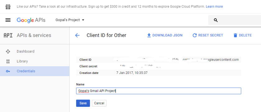
At first, we must create a Google API Console project. Once created, we get credentials for it. Credentials are essentially composed of the following two values that are known to both Google and the application.

  1. Client ID
  2. Client Secret

Google console pages look like below:

Google Console

Application Secret

Get access token

The second step is to get an access token from Google Authorization Server. During access token request, a scope parameter is also sent. Scope indicates all the accesses requested for.

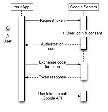
Depending on the kind of applications (web server, installed, client side) the authorization sequences might vary slightly. Since ours is an installed application, we would get authorization code first. We then exchange this code for a token. Below image that is taken from Google, depicts the process.

webflow

Get authorization code

To get authorization code from Google, we first open an HttpListener on local  loopback address, with a dynamically found available port. However, this requires elevated privilege. Hence, the application needs to run at elevated privilege. This could be avoided by doing URL reservation. However, that itself requires elevation.

We then open an authorization request in browser from the application. Authorization request would require:

  1. Authorization endpoint: https://accounts.google.com/o/oauth2/v2/auth
  2. Scope: https://www.googleapis.com/auth/gmail.modify
  3. Redirect URI: local loopback address, as explained earlier
  4. Client Id: Client Id credential, as retrieved for the Google API Console project
  5. State etc.: some additional information like state etc. to verify that response from server is due to a request made by this application. Verification happens once the response from Google server is back.

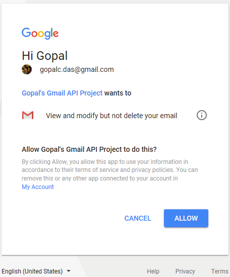
User’s consent screen looks like below.

Authentication picture

Scope can vary. Modify as scope, as shown here is sufficient to call all the three APIs (get, list and insert) that we need for our application. However, instead of asking for all the authorization upfront, scope should be increased incrementally.

If all is well, we will get an authorization code. However, to make any API call, we need access token. So now we have to exchange this code for a token.

We make an HttpWebRequest POST using

  1. Token endpoint: https://www.googleapis.com/oauth2/v4/token
  2. Code: as found earlier
  3. Client ID: credential as explained earlier
  4. Client secret: credential as explained earlier

All Gmail API endpoints are https, meaning all API calls have to be made using encrypted SSL/TLS channel. In .NET, we can easily use HttpWebRequest class. However, in other languages, if such a library is not available, we might use GnuTLS, OpenSSL etc. to create a TLS/SSL channel to enable us making https calls.

Make API call using access token

Now we can make Gmail API call, using the token in an authorization header.

Refresh Access Token

Access token has limited lifetime. We might require refreshing the access token, if necessary.

Getting emails from Gmail

To read emails, we will use list and get APIs, using the access token that we already received.

list

For list API call, we are making an HttpWebRequest GET request with endpoint: https://www.googleapis.com/gmail/v1/users/userId/messages.

Parameter userId is the gmail id. Optional query parameter q can be used, to specify after and before date to filter data. It should be mentioned that there is a max limit (I found it to be 500) as to how many emails (essentially, emaid id and thread id combination) we can read. We are content with as many results as found in the first call. No attempt is made to make further calls to read more emails.

get

For each listed email found in the above call we are now calling the get API using GET https://www.googleapis.com/gmail/v1/users/userId/messages/id.

Parameter userId is gmail id and id is the email id that is found from the previous call. Optional query parameter, format is used with value set to full. For each email, we are retrieving the subject and labels. If the input has a time component, then at this stage, we can further filter based on it, using internalDate property of the Users.Message resource.

Encryption

Encrypt with Rijndael

For encryption, Rijndael is used. Password and salt are taken as input. A 256 bit AES key is generated. We are using RijndaelManaged with default 128 bit block size; hence, it is AES compatible. Since this is symmetric key, the same key is used for both encryption and decryption. And the same key is used for all the emails.

get with format raw

For each email, we are making another call to get API, this time with format set to raw. Here we are duplicating the read API call. However, this way, we can directly get the raw property of Message resource, necessary to make insert API call. We don’t need to construct the raw property on our own.

At first, we are decoding the raw as found above. Then we are searching for the subject (that, we collected earlier, using get API with format full) in that. Starting from first character of the subject, we are encrypting the rest of raw. That will encrypt subject and body parts, along with some more data.

Regarding encryption, we could do that for the whole of raw or only for parts like subject, body and so on. As mentioned above, for simplicity, we have encrypted everything starting from subject. We have also written functions and tested that we can correctly decrypt the encrypted data.

While inserting the email into gmail folder, it would have been better if we could somehow indicate that the email is encrypted. That way, we could stop encrypting an email more than once, or identify that a certain email is in encrypted form.

So, in short, data in field raw of the Message resource is decoded, converted to a string and then encryption is applied on the plain text. It is then reverted back to base64url encoded form for insert.

Insert emails back

insert

The encoded raw along with labelIds collected earlier is now used to make an insert API call using POST https://www.googleapis.com/gmail/v1/users/userId/messages.

Once again, userId is the gmail id. Only raw and labelIds are used (in the request body), the latter (labelIds) is to make sure that the inserted email ends up in the same folder. Thread Id parameter could be used easily, however, chose not to include.

We have not used the upload URI. This is because we have only dealt with metadata and not (email) attachments, once again for simplicity.

Output

When the application runs, it asks user to press a key. Once the key is pressed, it starts working in asynchronous mode. Pressing a key further would stop it.

The application first opens Google server in browser for user to authenticate/authorize. Once that is done, it prints out how many emails it is going to read/encrypt/insert, based on the input parameters. It might take a while before it starts printing a line for each of the inserted emails.

This is how it looks in the Gmail folder.

Output.png

GMail API client libraries could be good starting point for writing such an application.

GitHub: GMail API

Index

Multithreaded Programming

32nd Friday Fun Session – 25th Aug 2017

Multithreading is a very important aspect of programming. Here we discuss some fundamental concepts and issues around it.

Process vs. Thread

A thread is a sequence of execution, a feature of operating system (OS). OS allocates processor time to a thread. Every process must have at least one thread. After all, it is a thread that executes the instructions.

Operating system gives each process some memory and it makes sure memory of one process is not accessible by other processes. However, all threads of a process would share its memory space, as the threads are parts of it.

Why do we need more than one thread?

As stated earlier, every process has at least one thread. Why do we need more than one thread? There are several reasons for that:

  1. Better UI experience: we can leave an exclusive thread to get user input, giving user a smooth interactive experience while having other threads to do other works.
  2. Do more things: with more than one processor available, using more than one thread, we can get more work done simultaneously.
  3. Use more things: different parts of software might be using difference resources of the computer. More than one thread can be used to simultaneously work with those resources.
  4. Doing slow things: sometimes we need to do some time consuming or slow thing, like writing to disk. We can create a separate thread to do that.

Concepts and Issues

We will focus on the following using VC++ concepts/terminologies/semantics:

  1. Types of threads
  2. Creating threads
  3. Memory issues
  4. Synchronizing threads
  5. Coordinating threads
  6. Exiting threads

Types of threads

There are two kinds of threads: user-interface (UI) thread and worker thread.

UI thread

UI thread has a message pump/loop that is nothing but an infinite loop that keeps on reading a message directed to the thread. Usually, PostThreadMessage is used to post (there is no corresponding send function) message to it. All these messages are queued in message queue, retrieved one by one and processed.

Since UI thread is in an infinite loop, it does not exit on its own. It has to be explicitly exited using PostQuitMessage.

UI thread can create UI components like showing a message box or other UI etc.

Worker thread

Worker thread does not have any message pump. That also means, it cannot receive any message. It cannot show any UI. It executes a set of instructions that is part of it and exits once execution finishes, meaning the thread does not exist any more after that.

Creating threads

AfxBeginThread function can be used to create both kinds of threads. However, a thread can be created in two modes: one that starts executing immediately; another that gets created in suspended mode and can be resumed later.

Each thread’s stack takes a 1 megabyte. 64 bit applications would fare better but keeping the number of threads low should be a priority.

Memory Issues

The thread can work on its own, allocating some (heap) memory that it will exclusively use. However, many a times, main process allocates some (heap) memory and passes it to a thread. This memory is usually freed up (to avoid memory leaks) by the process itself, as it allocated the memory at the first place. However, the process has to be careful not to free up memory when it is still being used by the thread. If the memory is deleted / freed and the thread is still accessing it, application/process/thread would crash (thread is part of the process).

That is one of the reasons we need to track the thread as to when it exits.

When we know that all threads that are using a certain memory have exited, we can free the memory. One way of doing this is again sharing/passing certain process (memory) flag to thread that it can use/set to indicate when it exits.

Synchronizing threads

In last section, we saw that process shares some memory with threads. At times, more than one thread might be using the same piece of memory. If multiple threads, running concurrently, access/modify common memory simultaneously, there would be data inconsistency and access violation crash. To deal with this we need to make those code segments as critical section. Access to critical section is to be controlled by synchronization techniques. There are a number of them. One light weight (compare to mutex etc.) intra-process technique (processor-specific test and set instruction) would be critical section (InitializeCriticalSection, EnterCriticalSection, LeaveCriticalSection, DeleteCriticalSection).

However, common memory object is not the only thing that we might need to synchronize.

Coordinating threads

One of the reasons, we create threads is to do some additional work. At times, one thread (main thread or a created one), let’s call it waiter, is waiting somewhere for another thread (main thread or a created one), let’s call it doer, to finish certain work. How would that be achieved?

We can use event based signalling mechanism. We can create an event (CreateEvent). A waiter can wait on it, usually using a blocking call (WaitForMultipleObjectsEx). Once doer is done, it can signal (SetEvent) using the event handle that it is done. Waiter would come out of the wait (blocking call) and it would know that the work for which it was waiting for is completed.

Waiter thread can again put the event to nonsignaled state (ResetEvent) and start waiting for the doer to signal it, and the cycle can go on and on.

An event can be either named or unnamed.

An event can also be created in two modes: manual-reset that requires an explicit (ResetEvent) call to put that event into nonsignaled state; another is auto-reset that creates the event with nonsignaled state.

Once we are done with an event, it should be closed (CloseHandle) else it would cause resource (handle) leak.

Exiting threads

When a process needs to exit, it should make sure that all the created threads are gracefully shut down first.

UI thread can be instructed to exit using PostQuitMessage function. However, it might take a while as there might be other messages in the queue. In that case, application should wait for the sake of a graceful shutdown. Otherwise, depending on what this thread is designed to do, the system might go to an unstable state, say, due to an inconsistent state of an inter-process synchronization object.

Since worker thread cannot be posted a message, we can use TerminateThread. However, once again this is a dangerous thing to do, for the same reason (can result in unstable state) as mentioned earlier.

So we need to be patient during shutdown. We can use the shared variable approach as discussed earlier, or an event based mechanism so that the process knows when all threads have exited.

Index

Solution – Scoring Weight Loss

29th Friday Fun Session – 4th Aug 2017

Given a sequence of weights (decimal numbers), we want to find the longest decreasing subsequence. And the length of that subsequence is what we are calling weight loss score. This is essentially the standard longest increasing subsequence (LIS) problem, just the other way.

This is the solution to JLTi Code Jam – Jul 2017 problem.

Let us walk through an example

Let us take the example as mentioned here: 95, 94, 97, 89, 99, 100, 101, 102, 103, 104, 105, 100, 95, 90. The subsequence can start at any value, and a value in a subsequence must be strictly lower than the previous value. Any value in the input can be skipped. The soul goal is to find the longest subsequence of decreasing values. Here one of the longest decreasing subsequences could be:  105, 100, 95, 90 and the length would be 4.

Even though, in our weight loss example, we have to find the length of longest decreasing subsequence, the standard problem is called longest increasing subsequence. Essentially the problems are the same. We can have a LIS solution and can pass it the negative of the input values. Alternatively, in the algorithm, we can alter the small to large, greater than to smaller than etc. We chose the former.

We will use two approaches to solve this problem: one is a dynamic programming based solution having O(n2) complexity, another is, let’s call it Skyline solution having O(n log n) complexity.

Dynamic Programming Solution

Let’s work with this example: 95, 96, 93, 101, 91, 90, 95, 100 – to see how LIS would work.

When the first value, 95 comes, we know it alone can make a subsequence of length 1. Well, each value can make a subsequence on its own of length 1.

When the second value 96 comes, we know it is greater than 95. Since 95 already made a subsequence of length 1, 96 can sit next to it and make a subsequence of length 2. And it would be longer than a subsequence of its own of length 1.

When the value 93 comes, it sees it cannot sit next to any value that appeared prior to it (95 and 96). Hence, it has to make a subsequence of its own.

When the value 101 comes, it knows that it can sit next to any prior values (95, 96 and 93). After all, it is bigger than each of them. It then computes the score it would make if it sits next to each of them, separately. The scores would be 2, 3, and 2, if it sits next to 95, 96 and 93 respectively. Of course, it would choose 96. The subsequence is 95, 96, 101 and the score is 3.

So we see, we can go from left to right of the input, and then for each of the previous values, it sees whether it can be placed after it. If yes, it computes the possible score. Finally, it chooses the one that gives it the highest score as its predecessor.

So we are using the solutions already found for existing overlapping sub-problems (the scores already computed for its preceding input values, that we can reuse) and can easily compute its own best score from them. Hence, it is called a dynamic programming solution.

The following table summarizes it.

DP table.png

There are two longest subsequences each with length 3. For a certain value, if we need to know the preceding value, we can backtrace and find from which earlier value its score is computed. That way, we can complete the full subsequence ending with this value.

Since for each of the input values we are looping all the preceding values, the complexity is O(n2).

Skyline Solution

In this approach, we would retain all incompatible and hence promising subsequences since any of them could lead to the construction of one of the final longest subsequences. Only at the end of the input we would know which one is the longest. Since we are retaining all incompatible subsequences I am calling it Skyline, inspired by Skyline operator.

It is obvious but let me state here, all these solutions are standard, already found and used. However, Skyline is a name I am using as I find it an appropriate term to describe this method.

If there are two apples: one big and another small, and if you are asked to choose the better one, you would choose the big one. However, if you are given an apple and an orange, you cannot, as they are incomparable. Hence you need to retain both.

When a value comes it can be one of the below three types:

Smallest value (case 1)

  1. It won’t fit at the end of any existing subsequences. Because the value is smaller than all the end values for all existing subsequences.
  2. There is no other way but to create a new subsequence with this value.
  3. We can safely discard all single value subsequences existed so far. After all, the new subsequence with the smallest value can be compared with each of them and it is clearly superior to them (score for each such subsequence is 1 and the end (and only) value for the new one is the smallest – hence it can accept more future input values than the rests).
  4. In the list of subsequences we can retain the single value subsequence at first. Meaning, every time the new smallest value comes, we simply replace the existing smallest value listed as the first subsequence.

Biggest value (case 2)

  1. The opposite of the previous case is: the new value is bigger than the end values of each of the existing subsequences.
  2. So it can fit at the end of all existing subsequences. So which one to choose?
  3. Suppose, it is the end of the input. In that case, we would like it to go at the end of the longest subsequence found so far and make it longer by one more.
  4. However, if it is not the end of the input and suppose there are some future input values coming that are bigger than the end value of the present longest subsequence and smaller than the present input value. By placing the present input value at the end of the present longest subsequence we will jeopardize a more promising possibility in future.
  5. So we should rather copy the longest subsequence found so far and add this new value at the end of it, making it the new longest.
  6. At the same time, we retain the previous longest subsequence as it is, that by now is the second longest subsequence.
  7. We will add this new and longest subsequence at the end of the list.

Middle value (case 3)

  1. We have a third case where the input value can fit the end of some subsequences and cannot fit at the end of the rest subsequences.
  2. This is because this new value is bigger than the end values of some sun-sequences and smaller than the same for the rests.
  3. So which one to choose? Of course, we have to choose one where it can fit, meaning from those whose end values are smaller than the input value.
  4. And we would like to choose one with the largest end element (yet it is smaller than the input value).
  5. However, we cannot just over-write it for the same reason as stated earlier (case 2, promising reasoning). Rather we copy it, add the new value at the end of it and add it to the list.
  6. Where – at the end of the list?
  7. No, we would insert in next to the subsequence from which we copied and extended it.
  8. And we can safely discard all other subsequences with the same length as this newly created  subsequence. After all, the length is the same and it’s end element is smaller than the end elements of the rests having equal length of it.
  9. Shall we run a loop over the list to find those to be deleted? No, we just need to find the next subsequence and if its length is the same as the newly created subsequence we delete it. No more checking is required.
  10. Why so? Please read the second point as stated below.

So we have handled all possible input values. The list of subsequences that we have created would have some nice properties:

  1. As we go from the first subsequence to the last in the list of subsequences, the length will gradually increase.
  2. There would be a maximum of one subsequence with a certain length.
  3. To find whether the input value is a case 1 or case 2 or case 3 type, we can easily run a binary search with O(log n) complexity over the end elements of the subsequences in the list. Since we would like to do so for each of the n input values, the complexity of this approach would be O(n log n).
  4. For doing the above we can use the list, just that we need to look at the end elements. Then why are we retaining the complete list?
  5. The answer is: to output the longest subsequence as well.
  6. Could we do it without saving the complete subsequence?
  7. We leave it for another day.

Walking through an example

Let’s go through the same example as used earlier: 95, 96, 93, 101, 91, 90, 95, 100.

95 (case 1)

95

96 (case 2)

95

95, 96

93 (case 1)

93

95, 96

101 (case 2)

93

95, 96

95, 96, 101

91 (case 1)

91

95, 96

95, 96, 101

90 (case 1)

90

95, 96

95, 96, 101

95 (case 3)

90

90 95

95, 96 (deleted)

95, 96, 101

100 (case 3)

90

90 95

90 95 100

95, 96, 101 (deleted)

Once all the input values are treated, the last subsequence would be the longest one.

GitHub: Scoring Weight Loss

Index

Solution – Manipulating Money Exchange

25th Friday Fun Session – 7th Jul 2017

Given a set of currencies and some exchange rates among them, we want to find if there exists an arbitrage; meaning, if it is possible to exploit the discrepancies in the exchange rates and transform one unit of a certain currency to more than one unit of the same, thus making a profit.

This is the solution to JLTi Code Jam – Jun 2017 problem.

Let us walk through an example

Let us take the example as mentioned here. We can start with 1 USD, convert that to SGD (1.380 SGD), then convert that to MYR (1.380 * 3.080 MYR), then convert to INR (1.380 * 3.080 * 15.120 INR), then convert to GBP (1.380 * 3.080 * 15.120 * 0.012 GBP), then convert that back to USD (1.380 * 3.080 * 15.120 * 0.012 * 1.30 = 1.0025503488 USD).

We end up with more than 1 USD. That means, we have an arbitrage in this set of exchange rates. The profit making cycle here is: USD -> SGD -> MYR -> INR -> GBP. And since it is a cycle, we can start from any currency within it. For example, SGD -> MYR -> INR -> GBP -> USD also represents the same cycle.

The transformation

In general, if we have to make a profit, the respective rates in the cycle, when multiplied, should give more than 1, as we have seen in the above example.

Formula

Negative cycle in Bellman-Ford

After some simple transformation of the profit making condition, we see, if we take negative of log rate, and use that as the edge cost/distance, then finding profit making cycle is equivalent to finding negative cycle in the corresponding graph. And we can do so using Bellman-Ford algorithm.

To be precise, each of the currencies would be considered as a vertex. If there exists an exchange rate r between two currencies then there would be a directed edge between the corresponding vertices, and –log r would be the associated cost/distance of that edge.

Source of Bellman-Ford

The next question comes: using which vertex as source shall we run the Bellman-Ford? Let us see the below graph.

Souce.png

Suppose, we have a single profit making cycle here: GBP-> AUD -> CAD. In that case, if we start with USD as source vertex, we will never detect this cycle.

Add extra currency as source

To solve this problem, we need to add an extra currency, and then create edges from it to all the existing currencies with cost 0. Now using this extra vertex (EXT) as source we have to run Bellman-Ford and that would ensure that we can detect a cycle, if there exist one.

Extra Souce

GitHub: Manipulating Money Exchange

Index

Models in Machine Learning

15th Friday Fun Session (Part 1) – 28th Apr 2017

Usually, machine learning algorithms build a model. We are trying to understand what a model looks like and some associated concepts around it.

Descriptive vs. predictive analytics

Descriptive analytics looks at historical data to understand what happened. It describes historical data using different statistical techniques and visualization.

Predictive analytics looks at historical data to understand and predict future. It also uses different statistical techniques, machine learning algorithms etc.

Both can have models, called as descriptive and predictive models. Here by model we are referring to predictive model.

Understanding model

The globe of the Earth does not show every detail of it but this small model can be put on our desk and it can give us an idea as to how the Earth looks like. When we talk about machine learning model, it is similar to that. It represents the data that is used to build it.

Suppose we have some employee data as shown in the table below.

Training Data.png

We want to build a model using this data set. Later, given an employee’s salary and experience, we would like to know her designation, using it.

Model as logical statement or rule

Based on the above data, we can construct two logical statements as shown below.

If salary is more than 3,000 and experience is more than 5 years 
then the employee is a Senior Software Engineer.

Otherwise, the employee is a Junior Software Engineer

Given an employee’s salary and experience, we can find her designation by using the above formula. That formula is called the model.

Model as function

The formula can take the form of a function as well. Let us draw a function that can work as a model for the above data set.

Function Model.png

We have used X-axis for experience, and Y-axis for salary (in thousands). The three data points would be placed as shown above.

The red line can work as a model. All employees on the left side of it, shown as green points are Junior Software Engineers. And all employees on the right side of it, shown as blue points, are Senior Software Engineers.

Note that, this model is not an exact translation/equivalent of the earlier model expressed as logical statements. Meaning, the same input data might be classified (Junior Software Engineer or Senior Software Engineer) differently.

The (red) line equation can be written as

   x + y = 5
=> x + y - 5 = 0
=> f(x, y) = x + y - 5

The model can be expressed this way:
if f(x,y) >= 0, then Senior Software Engineer
if f(x,y) < 0, then Junior Software Engineer

If a new employee input comes with salary 4,500, and experience 1 year, this model would classify her as a Senior Software Engineer.

   f(x, y) = x + y - 5
=> f(x,y) = 4.5 + 1 - 5
=> f(x,y) = 0.5
=> f(x, y) >= 0

If we use the earlier model to classify this input, it would classify it as Junior Software Engineer – different prediction!

Hybrid model

A model can use a combination of both logical statement and function.

To summarize, a model can be expressed using logical statement, function or a hybrid of both.

When a model is built?

At the beginning when we have some data, usually we split it into training data and test data; we provide the training data to a machine learning algorithm that in turn builds a model. Then we use the test data to check how this model is performing and tune the model, as and if required. The model can be further updated, say, periodically, when more data is gathered.

Different machine learning algorithms build different kinds of model. Some build at first, some delay it.

Eager vs. Lazy learning

When a machine learning algorithm builds a model soon after receiving training data set, it is called eager learning. It is called eager; because, when it gets the data set, the first thing it does – build the model. Then it forgets the training data. Later, when an input data comes, it uses this model to evaluate it. Most machine learning algorithms are eager learners.

On the contrary, when a machine learning algorithm does not build a model immediately after receiving the training data, rather waits till it is provided with an input data to evaluate, it is called lazy learning. It is called lazy; because, it delays building a model, if it builds any, until it is absolutely necessary. When it gets training data, it only stores them. Later, when input data comes, only then it uses this stored data to evaluate the result.

There is a different set of pros and cons associated with eager and lazy learning. It is obvious that lazy learning would take less time during training but more time during prediction.

Eager learning builds a model for the whole data set, meaning it generalizes the data set, at the beginning. It might suffer accuracy compare to lazy learning that has more options in terms of the availability of the whole data set as well as the mechanisms to make use of it.

Lazy learning is typically divided into two types: instance-based learning and lazy Bayesian rules.

Instance-based learning

Do all machine learning algorithms build a model?

No, all machine learning algorithms don’t build a model, when by model we mean generalizing the data. For example, decision tree builds a model but k-NN does not.

A row is also called an instance, meaning a set of attributes. Hence a set of training data is also called a set of instances. When a machine learning algorithm does not build a model, rather uses the set of instances directly to evaluate the result, it is called instance-based learning. It is also called memory based learning as it memorizes the whole data set. For the same reason it is also called rote learning.

Instance-based learning, as mentioned above is one kind of lazy learning.

Supervised, unsupervised and semi-supervised learning

The employee example that we have discussed here is an example of supervised learning. Here we wanted to predict an output variable – designation of an employee by providing input variables – salary and experience. While building the model, we provided training data having most (all for the example here) values for input variables and all values for the corresponding output variable.

An important requirement of supervised learning is that, for all the training data we must provide the output variable value. Because, supervised learning learns from it. Most machine learning algorithms use supervised learning.

However, some machine learning algorithms don’t predict an output variable. They just take only the input variables and try to understand, say the distribution or pattern of the data. They are classified mainly into clustering and association rules. For example, when we do clustering, it might come up and say the given data falls into 3 groups.

There is a third type of learning, in the middle of supervised and unsupervised, called semi-supervised. In many real life examples, a good portion of the training data does not have labels for the target variable, meaning many instances of the training data don’t have the output attribute value known. It might be expensive to label them as it might require domain experts.

In this situation, unsupervised learning comes to rescue. It labels them, and then the labelled data is fed into supervised algorithm (to build model) for prediction. This process (unsupervised algorithm labels them and supervised algorithm predicts), might be repeated unless satisfactory accuracy is acquired.

In the above example, we have seen examples of supervised models. However, predictive models include unsupervised and semi-supervised models as well, the latter being a combination of supervised and unsupervised models.

Parametric vs. non-parametric model

Some machine learning algorithms would come up with a model with a predetermined form. For example, it would construct a function with 2 parameters. Now given the training set it would compute that two parameters and come up with a function. An example would be naive Bayes. They are called parametric. For prediction they would depend on this function alone.

On the other hand, some machine learning algorithms would construct a model based on the information derived from the data. For example, k-NN, C4.5 – a decision tree etc. They are called non-parametric. Non-parametric does not mean no parameter, rather no predetermined parameters.

k-NN as an example of a non-parametric model might create a little confusion as k-NN does not build any model at the first place. Well, here model is used in a broader sense to mean how it computes output value. K-NN uses the complete training data set to do so. Hence the whole training data set is the input parameter. Adding one more training data can be thought as increasing the parameter by one. That perfectly matches another definition of non-parametric model that says – the number of parameters grows with the amount of training data.

Classification vs. regression

The model that we are discussing so far – given salary and experience, predict the designation, is called a classification model. The reason is the output variable, designation – a categorical variable. Meaning, it would take one of the predefined categories or classes. In this example, there are two categories or classes: Junior Software Engineer and Senior Software Engineer.

Let us alter the input and output a bit for the model. Suppose the model would now predict the salary, given experience and designation. Then this model would be called a regression model. The reason is the output variable, salary – a continuous variable. Meaning, it can take any value, not limited by a predefined set of classes, unlike earlier example.

Bias vs. variance

Let us continue with the previous example of the model that predicts salary. Ideally, the salary would be calculated by taking the input values, experience and designation into consideration.

But assume the model that is built by a machine learning algorithm, is so simple and dumb. Let us say, given the training data, it computes the average of the salary (2500 + 5500 + 6200) / 3 = 4733 by ignoring all other parameters. Now when an input comes asking the salary, it does not care the experience or designation of the input. The only output (salary) that comes out of it is 4733. Now that is called a highly biased model. It generalizes the data so much that it ignores the input values of the training data and hence underfits the training data. A biased model that does not distinguish a 2 years experienced Junior Software Engineer from a 15 years experienced Senior Software Engineer, and predicts the same salary of 4733 for both, is not a good model, for obvious reasons.

By the way, what machine learning algorithm can possibly come up with such a model and under what condition?

On the other extreme, there is this model with high variance that considers each minute detail of the training data that is possibly nothing but noise, to be the ultimate truth and incorporates them into the model. Hence it is said to be overfitting the training data, and results in a highly complex model. However, a model with all these intricate truths of training data, even though performs very well with training data (after all, the model is built to overfit the training data), do not stand the test of real world. This kind of model, with highly fluctuating prediction, due to little changes in input parameters, is not desirable either.

What we need is a balance, a trade-off between bias and variance; achieving which is a prerequisite, for a good model.

Index

Synchronizing Web System

22nd Friday Fun Session (Part 3) – 16th Jun 2017

When we have to implement an idempotent operation in web application, where the respective method execution is not idempotent when executed simultaneously, it is essential that we use concurrency control. Here we focus on .NET application deployed in IIS.

Idempotent operation

Suppose user requests to approve a certain transaction, say, transaction Id 100, hence it is data specific. We need to make sure this is an idempotent operation, meaning, no matter how many times the request comes, simultaneously or serially, the end result should be the same.

Concurrency and thread synchronization

If more than one request comes, from the same user or from multiple users simultaneously, we have seen IIS might launch multiple threads, one for each request. It is possible that they are executed simultaneously.

Let’s take a closer look. Suppose the two requests were initiated at 12:00:00:000 PM. The requests ended up in IIS at 12:00:01:000 PM, two threads starts processing them at the same time at 12:00:01:001 PM. Both the threads find that the transaction has not been approved yet, and proceed to do the same thing, like send an email, make some database entries etc. At the end both mark that the transaction is approved.

So we see that, what was supposed to be an idempotent operation has ended up sending two emails and so on, clearly failing to be one. If we don’t have any concurrency control in place, nothing is stopping from sending two emails from the two threads. After all, both the threads are executing simultaneously checking, finding and doing the same thing, at the exact same time.

Concurrency control is essential here. That means, at the beginning we need to place a gate through which only one thread can enter, at a time. Once it enters, it should mark that it is approving a certain transaction. Then all other threads who would enter the gate later serially (one after another), can detect that somebody else is processing that exact same request and quit gracefully.

Intra-process synchronization

We will walk through some options, even though they would not qualify to be the desired solution. We would do so just to explain the issues around the options, so that we can rationalize the final solution(s).

Let us start with lock, provided by C#. lock can implement critical section, meaning it can make a certain portion of the code executable only by one thread at a time. So the transaction processing method can be wrapped using a lock. That will make sure only one thread of a process is executing the method at any given point of time.

However, we have two issues here:

First, we are locking the whole method. We wanted to make sure only transaction Id 100 gets approved only by one thread at any point of time. But we end up blocking approval for all other transactions, say, transaction Id 99 or 101, when approval for transaction Id 100 is going on.

We can solve this issue by implementing a named lock, meaning the lock will have a name, say, TranApproval_100. That way, only threads executing approval requests for the same transaction will be executed serially. Instead of using lock, we can achieve the same using interned string, named mutex etcas well.

Second, the scope of the lock is within the process. Nobody outside the process knows about it. However, we know that in web garden configuration, there might be more than one process running for the same web application and the two threads can come from two different processes. In that case, the thread in the first process would not know that the thread in the second process is having a lock. Hence both the threads would happily execute the same method simultaneously. We can solve this problem by using named mutex, an inter-process synchronization mechanism.

Inter-process synchronization

We see that using a named mutex, say, the name of the mutex is TranApproval_100, we can make sure we don’t block approval for other transactions. Meaning only thread approving transaction Id 100 will execute, without blocking approval for, say, transaction Id 99 or 101.

We also see that between the two threads running in two processes in web garden configuration, only one would do the approval and other would quit. This is because the named mutex is visible to all processes throughout the operating system.

However, we also know that in web farm configuration, the two processes, executing the two threads, both intending to serve the approval processing for transaction Id 100, might be running in two different web servers. In such a case, this inter-process synchronization mechanism that we just explored, would not work.

External and Common

So we see that we have to use something that is both external and common to web servers. If we have one common database that is used by all the processes then we can use something from the database to make sure that the threads are processing the requests one by one.

Using transaction within application

Using the concurrency control support provided by database, we can make sure only one method is doing the database operations, at any point of time. If we are using ORM, say Entity Framework, then we can use the transaction support provided from version 6 onwards (Database.BeginTransaction(), Commit, Rollback etc.). Since we want them execute serially, we know we have to use serializable isolation level System.Data.IsolationLevel.Serializable. We can begin the transaction with this isolation level parameter.

There are two problems associated with this. First, we are again serializing the whole transaction approval process, meaning blocking approval for transaction Id 101, while processing the same for transaction Id 100.

Second, we cannot stop non-database operations like sending email etc.

Named synchronization using database

The first problem can be solved by, as we have seen previously, using a named synchronization mechanism. The second problem can also be solved using the same, but we need to make sure we are using the synchronization mechanism to serialize the whole method, not just the database transaction.

Named lock table

We first create the following table that will keep track of the transactions, presently under processing.

CREATE TABLE [Web].[LockInfo]
(
  [LockInfoId] [int] IDENTITY(1,1) NOT NULL, 
  [LockName] [nvarchar](256) NULL, 
  [DurationInSeconds] [int] NULL, 
  [CreatedOn] [datetime] NOT NULL, 
  CONSTRAINT [PK_LockInfoId] PRIMARY KEY CLUSTERED 
  ( 
    [LockInfoId] ASC
  )
  WITH (PAD_INDEX = OFF, STATISTICS_NORECOMPUTE = OFF, 
  IGNORE_DUP_KEY = OFF, ALLOW_ROW_LOCKS = ON, ALLOW_PAGE_LOCKS = ON) 
  ON [PRIMARY]
) ON [PRIMARY]

GO

ALTER TABLE [Web].[LockInfo] ADD  DEFAULT ((60)) FOR [DurationInSeconds]
Lock name

LockName is the name of the lock, like TranAproval_100.

Duration

We should not hold the lock forever. If after acquiring the lock things go wrong, for example, the caller somehow misses to unlock it or there is a crash, this resource cannot be locked again by any thread in future. The created date along with the default duration of 1 minute would make sure, after a minute this lock becomes invalid. This is based on the assumption that approval processing would be done within a minute.

Using stored procedure

We create the following stored procedure.

CREATE Procedure [Web].[usp_Lock] 
  (@Lock BIT, @LockName NVARCHAR(256), @LockDuration INT = NULL) 
  AS 
    BEGIN SET TRANSACTION ISOLATION LEVEL SERIALIZABLE 
    BEGIN TRY 
      BEGIN TRANSACTION 

      DECLARE @Success AS BIT 
      SET @Success = 0

      IF(@Lock IS NULL OR @LockName IS NULL) 
      BEGIN  
        SELECT @Success AS Success; 
        ROLLBACK TRANSACTION
        RETURN; 
      END 

      IF(@Lock = 1) -- LOCK
      BEGIN 
        DELETE FROM [Web].[LockInfo] 
        WHERE @LockName = [LockName] AND 
        DATEADD(SECOND, [DurationInSeconds], [CreatedOn]) < GETUTCDATE();

        IF NOT EXISTS (
                       SELECT * FROM [Web].[LockInfo] 
                       WHERE @LockName = [LockName]) 
        BEGIN 
          IF(@LockDuration IS NULL) 
            INSERT INTO [Web].[LockInfo]  
            ([LockName], [CreatedOn]) 
            VALUES(@LockName, GETUTCDATE()) 
          ELSE 
            INSERT INTO [Web].[LockInfo]  
            ([LockName], [DurationInSeconds], [CreatedOn]) 
            VALUES(@LockName, @LockDuration, GETUTCDATE())
          
          SET @Success = 1 
        END 
      END 
      
      ELSE -- UNLOCK
      BEGIN 
        DELETE FROM [Web].[LockInfo] 
        WHERE @LockName = [LockName] 
        SET @Success = 1 
      END 
      
      COMMIT TRANSACTION 
    END TRY
  
    BEGIN CATCH 
      SET @Success = 0 
      IF(@@TRANCOUNT > 0) 
        ROLLBACK TRANSACTION
    END CATCH;
 
    SELECT @Success AS Success; 
  END

Lock and unlock

This stored procedure can be used for both lock and unlock operation of a named resource. The lock can be acquired for a given interval. In absence of any duration parameter, default duration of 1 minute will be used.

Leveraging isolation level

We make sure that this stored procedure can be executed serially, thus making sure only one transaction execute, at any point of time.

Here we focus on making the lock/unlock function faster, compromising concurrency by using the highest isolation level.

Leveraging consistency

We could have used unique constraint on lock name column in the Web.LockInfo table. In that case, we could use the default READ COMMITTED isolation of MS SQL Server, in the stored procedure, increasing concurrency. If a second thread would want to take the lock on the same resource, it would try to insert a row with the same lock name, resulting in failure, due to the unique constraint checking.

Performance

The two have different performance implications that we explain using an example.

Suppose two threads started executing simultaneously. The faster stored procedure takes one millisecond to execute. The first thread takes one millisecond to lock and then 100 milliseconds to execute the main approval processing, taking a total of 101 milliseconds.

The second stored procedure would wait one millisecond for the first stored procedure to lock. Then it would take one more millisecond to check that it is already locked, and hence it would take a total of 2 milliseconds to quit the processing.

On the other hand, suppose the stored procedure using default isolation level and unique constraint takes 3 milliseconds to lock. The first thread would take 103 milliseconds to execute.

The second thread that starts at the same time would take 3 milliseconds to fail while acquiring the lock and quit.

Based on the load and usage pattern, an appropriate mechanism can be chosen.

Usage for general purpose locking

This mechanism can be used not only for synchronizing transaction approval but all other cases that use named resources. Based on the load, more than one lock table (and/or stored procedure) can be used, each supporting certain modules.

GitHub: Named Resource Lock

Index

Interpreting IIS Internals

22nd Friday Fun Session (Part 2) – 16th Jun 2017

We are trying to understand how an HTTP request is processed by .NET web application, hosted in IIS in various scenarios with a focus on synchronization of the processing of that request. To be precise, we are interested in the thread and process contexts involved while serving an HTTP request.

Client request

Multiple clients across the globe, using their respective browsers, sending HTTP request to the web server.

Web server

All these http requests are ending up in IIS web server, hosting the application.

IIS kernel mode

In web server, HTTP listener, a kernel mode device driver, part of network subsystem, and part of the IIS – kernel mode of IIS to be precise, called http protocol stack (Http.sys), listens for http requests.

HTTPS.sys, as a forwarder, might directly pass the request to the right worker process, or as a request queuer, queues it unless a worker process picks it up. Once the response of that request reaches to it, it returns that back to client browser. Also as a kernel level cacher, it does some kernel level caching and if possible, returns the cached output directly, without involving any user level processing.

Worker process

Worker process, w3wp.exe, an executable, a process to OS, runs inside IIS user mode, is little different than other processes in the operating system (OS), in the sense that it can contain multiple application domains.

Application domain

Application domain represented by AppDomain object, a .NET concept, is a virtual process within a process. As said, it runs within a worker process. One application domain does not share its static variables etc. with another application domain running within the same worker process.

Usually, all static variables etc. of a process are visible to all within a process. It is not the case for worker process. This is how worker process is a special process, where one or more application domains are running inside it, as if each of them is a separate process, providing isolation. So what usually we are used to thinking as per process, in the world of IIS, inside worker process, it is actually per application domain.

Why Application domain, you might ask. Well, a web server can have many applications. Creating one worker process for each of them will end up creating many processes that is quite expensive. Creating an application domain for each of them and putting them together inside a single process is much cheaper.

Note that, one of the application domains can be stopped without affecting other application domains inside a worker process.

Worker thread

When worker process receives a request, it uses worker thread to process that request. If two users send two requests to the same web application, both of them can be simultaneously executed by two worker threads and served.

At any point of time, a worker thread can only be executed within a single application domain. An application domain can have multiple worker threads. But these worker threads are not confined to a single application domain. Rather they belong to worker process. When a thread is done with serving a request for a particular application domain, it is freed. At a later point of time, the same thread can be used to serve another request, belonging to a different application domain.

Web application

We develop web application. We are interested to know how this ending up running in IIS environment. Application domains are associated with web application. One web application has typically, one application domain running inside a worker process. One worker process might be running many application domains, each supporting a separate web application.

Application pool

Application pool is the container for (web) applications. Every application has to be assigned to a single application pool. A number of web applications can be assigned to a single application pool. But as mentioned earlier, a single application cannot be assigned to multiple application pools. All applications belonging to an application pool share the same configuration.

Worker process runs inside the application pool.

Application pool can be recycled, restarted. Applications belonging to other application pool are not affected by this. Thus application pool provides isolation.

So we see that a number of applications are contained within an application pool. And then a worker process running inside an application pool is again running a number of application domains, each application domain serving a different web application. Thus, we have two different levels of isolation.

Web garden

How many worker processes can be there inside an application pool? Well, it is configurable. By default, it is only one worker process running inside an application pool, supporting multiple web applications, by creating one application domain for each of the applications. And all these application domains are running as separate processes within that single worker process.

However, application pool can be configured to run more than one worker processes. In that case, it is called a web garden. In this situation, multiple worker processes can be running in a single application pool. Each of these worker processes, once again running multiple application domains, each belonging to one application.

In this scenario, each of the worker processes can have its own application domain for the same application. In other words, for a certain web application, we can have multiple application domains, each running in a separate worker process, all in the same application pool. To be precise, one application or web site can have multiple instances running in a single web server, if web garden is enabled.

This is important as it renders uses of static variables, application-wide variables etc. problematic in web application.

Web farm

When one web server is not enough to serve the clients requests, we need more of them to host the same application/web site. We call it web farm.

A load balancer would sit in front of the web servers and its IP will be exposed to external world. HTTP requests will come to load balancer first and it will then distribute the load to different web servers.

Individual web server can share the same database or replicated/partitioned database.

In a nutshell

Single server, application pool running one worker process

So we see that, multiple https requests for the same web application would be simultaneously served by multiple threads. Those threads can be executed within a single application domain belonging to a single worker process. This happens when only one worker process is set to run for an application pool.

Simple.png

In the above image, we see IIS having two parts – system and user mode. HTTP.sys is in kernel mode, forwarding HTTP request to 3rd application pool, belonging to application X. We further see that a single worker process inside that 3rd application pool is running two application domains X and Y. Two threads within application domain X – Thread 1 and Thread 2 are serving the two requests, respectively. The response will go back to client browser through HTTP.sys.

Single web server, application pool running more than one worker process, called web garden

Or the threads can come from different application domains associated with the same web application or web site, running inside different worker processes, all contained within the same application pool. This can happen in web garden configuration, where multiple worker processes are allowed to execute within a single application pool. We can understand any locking mechanism that works within a single process would not work in this setup. We would need to implement an inter-process synchronization mechanism, if our application is deployed in web garden.

Web Garden

In the above image, showing web garden, two requests are being served by two worker threads, belonging to two application domains (both associated with same web application), each running in a separate worker process, both of them (worker processes) contained within the same application pool.

Multiple web servers behind load balancer, called web farm

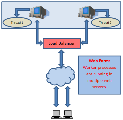
Or the threads can come from different physical web servers. This can happen in a web farm scenario, where multiple web servers sit behind a load balancer. We can understand that an inter-process synchronization mechanism, which works across the processes within an OS, would not work here. Since we have multiple web servers here, each running its own OS, inter-process synchronization mechanism would not work for application-wide synchronization.

Web Farm.png

In the above image, showing web farm, two requests are being served by two worker threads, each running in a separate web server.

Index