Incision into Isolation Levels

22nd Friday Fun Session (Part 1) – 16th Jun 2017

We are trying to see how isolation level, serializable to be precise, can help us implementing a synchronization mechanism for web application.

Let us start with ACID

ACID stands for Atomicity, Consistency, Isolation and Durability. It is detailed in ISO standard. Database systems implement this so that a sequence of operations, called as transaction, can be perceived as a single logical operation.

Atomicity

All operations of a transaction are all done or nothing done. Logging with undo capability can be used to achieve this.

Consistency

Given that all database constraints (foreign key, unique etc.) are valid at the beginning, the same should be maintained, at the end of the transaction as well.

Durability

All changes done by a committed transaction must go to storage even if database system crashes in the middle. Logging with redo capability can be used to achieve this.

Why Logging?

We talked about logging and then redo/undo in the previous sections. Why Logging? Well, when some transactions changes data, they are not immediately written to disk. Rather those pages are marked as dirty. Lazy writing flushes them to disk later. Instant writing to disk is expensive. Instead, logging the operation that is directly written to disk immediately, is much cheaper.

However, performance, while important is not a must. Logging is essential to ensure atomicity and durability. Any modification must be written to log before applying to actual database. This is known as write-ahead logging (WAL) This is to make sure that in case of a crash (say, 2 out 5 operations of a transaction are written to database storage and then it crashes), system can come back, read the log and figure out what was supposed to be done and what was not supposed to be done. By redoing and undoing necessary operations, durability and atomicity is ensured.

Focus on the I of ACID

Today we focus on the I of ACID, called isolation. When we are writing a transaction, we write the operations inside it thinking nobody else is doing anything else to the data that we are dealing with. Isolation property defines such an environment and database systems implements that.

So, why do we need such an environment? Well, without this, in a highly concurrent transaction execution environment, our understanding of the data we are working with will not hold true, as other would change them simultaneously. It will happen largely due to three problems: dirty read, non-repeatable read, and phantom read.

However, creating such an isolated environment is expensive in terms of performance. Hence, a number of other isolation levels are introduced, giving various degrees of isolation rather than a complete isolation.

The ISO standard defines the following Isolation levels that we will describe in terms of two transactions T1 and T2 that executes in parallel.

Read Uncommitted

Transaction 1 (T1) updates salary for Joe
Transaction 2 (T2) reads updated salary for Joe
T1 aborts transaction

We see that, T2 read dirty (because T1 did not commit the updated salary) data and went ahead with his decisions/operations inside it based on it, that was of course a wrong thing it did.

As the name implies Read Uncommitted reads uncommitted data, also called dirty data that is wrong. So we see, this isolation level does not guarantee isolation property and it is an example of a weaker isolation level. Note that along with dirty read, it also has non-repeatable read and phantom read problems.

Read Committed

The next better isolation level, as the name Read Committed implies, reads only committed data and solves the dirty read problem encountered previously in Read Uncommitted isolation level. Let us see through an example. Now T1 is running in Read Committed isolation level.

T1 reads the salary of Joe
T2 updates the salary of Joe and commits
T1 reads the salary of Joe

So we see T1 reads the salary of Joe twice, and it is different in the two cases. In the second case, it reads the data that was modified and committed by T2. No more dirty read by T1. Good.

But the isolation property expects each transaction to happen in complete isolation, meaning it would assume it is the only transaction that is taking place now. Joe’s salary was not updated by T1. Then why should T1 see different data when it reads the second time?

So we see, T1 could not repeat a read (the same salary for Joe). Hence, this problem is called non-repeatable read. Read Committed, like Read Uncommitted is another weaker isolation level. Again, note that, along with non-repeatable read it also has the phantom read problem.

Repeatable Read

To solve the non-repeatable read problem, Repeatable Read isolation level comes into picture. Since T1 reads the salary of Joe, no other transaction should be able to modify Joe’s data if we run T1 in Repeatable Read isolation level.

If we repeat the previous transactions we did earlier we would see T2 waits for T1 to finish first. Because T1 would use the right locks on the rows it reads so that others cannot delete/modify it. Repeatable read is solving the non-repeatable read problem as the name implies.

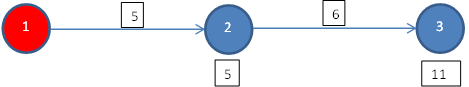
However, that won’t stop new data insertion. After all, Repeatable Read put necessary locks only on the data that it has read, not on future data. Hence, we will see ghost/phantom data. Let’s see an example.

T1 reads 4 rows in employee table
T2 inserts one record in employee table and commits
T1 reads 5 rows in employee table

We see that T1 sees a phantom row (the newly inserted row by T2) in its second read of employee table. Repeatable Read, once again, another weaker isolation level.

Serializable

So far, we see different isolation levels providing different degrees of isolation level but not what I of ACID really defines as isolation. We also know that weaker isolation levels are introduced to avoid the performance penalty that occurs for executing transactions in complete isolation. But at times, it becomes an absolute necessity to execute transaction in full isolation. Serializable comes into picture to implement that complete isolation. In serializable isolation level, it is ensured that we get the effect as if all transactions are happened one after another, in the order they started.

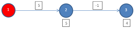
So if we rerun the earlier two transactions, we would see T2 waiting for T1 to complete first. Hence both the reads of T1 would read 4 rows. Only after T1 is done that T2 would insert a new row.

This solves all the three problems: dirty read, non-repeatable read and phantom reads.

At this point, it can be mentioned here that ISO standard expects serializable, not serial. The end result of a serializable execution is to produce a result equivalent to executing them one after another. Serializable does not necessarily executing transaction one after another, just that the end result is the same, had they executed serially.

MS SQL Server implementation

With Serializable, we are done with the 4 ISO transaction isolation levels. MS SQL Server implements all of them. In addition, it implements a fifth one, called Snapshot.

Snapshot

It is an isolation level that solves all the three problems just like serializable. So, why do we have two isolation levels doing the same thing? What special thing snapshot is doing?

If we closely observe the earlier serializable isolation level, implemented using locks, we see that it is too pessimistic. T2 has to wait for T1 to finish. But T2 could be simultaneously executed. After all, T1 is only reading, not modifying any data.

Snapshot comes into picture with optimistic concurrency control. It uses multiversion concurrency control (MVCC) to implement this. Every transaction starts with the latest committed copy it sees and keeps on executing the operations inside it.

So, for the last example we saw, in snapshot, T1 would read 4 rows in both the reads. After all, it had its own private copy. On the other hand T2 would start with its own copy, add a row in the middle. At the end, it would see there was no conflict. This is because no other transaction, T1 in this case, did anything conflicting. So, two transactions are simultaneously executed without violating the requirements of a serializable solation level.

What would happen if both T1 and T2 modify the same data, creating a conflicting situation? Well, both the transaction started with its own copy hoping that at the end there would no conflict, hence it is called optimistic. But if there is a conflict, the one committed first would win. The other would fail and rollback.

By the way, even though it is called serializable, write skew, anomaly is still present and it cannot be called serializable in ISO definition.

Database needs to be configured, which at times takes a while, to use this isolation. Again, since each transaction uses its own private copy, it is resource intensive.

At a glance

Isolation levels

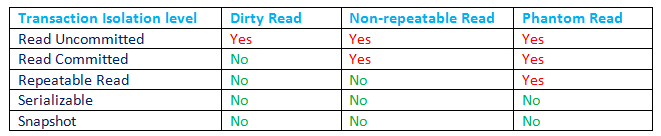
Default transaction isolation level for MS SQL Server

Read Committed is the default isolation level set for MS SQL Server. Keeping performance in mind, it is done this way. So all along if you had thought, by default, you were getting the I of ACID by SQL Server, you are wrong. You are living with non-repeatable read and phantom read unless you have explicitly changed the isolation level or used locks.

How to set isolation level in MS SQL Server?

We can set one isolation level at a time using the following command:

SET TRANSACTION ISOLATION LEVEL 
   { READ UNCOMMITTED 
   | READ COMMITTED 
   | REPEATABLE READ 
   | SNAPSHOT 
   | SERIALIZABLE 
   } 
[ ; ]

As mentioned earlier, to set snapshot isolation level some database specific configuration is required before executing the above command.

How long isolation level remains active?

Once set, it lasts for the session, the duration of which is largely controlled by the component that creates it. When another session starts, it starts with the default Read Committed.

Transaction

It is obvious yet important to remember, isolation levels works on transaction. After all, it is called transaction isolation level. If we want to isolate (using isolation level) the execution of a set operation as a single logical operation, then they have to be wrapped with Begin and Commit transaction.

Index

Maximum Subarray Problem

21st Friday Fun Session – 9th Jun 2017

Maximum subarray finds the contiguous subarray within a one-dimensional array having the largest sum.

Visualizing the divide and conquer solution

For the time being, let us forget about maximum subarray problem and focus on the divide and conquer solution that we discussed in the previous session.

If we visualize the tree, we see that from the left subtree the smallest value is propagated upwards.  On the way up, it is treated as the buy value and the right side values are treated as sell values. This way profits are calculated and maximum among them is retained. So we see two themes of processing as we go from left to right of the array:

  1. Retain the minimum value and treat it as the buy value.
  2. Calculate profit by treating each value seen as we go right and retain the maximum profit.

DP1.png

The above table shows day number in first row and the corresponding stock prices in second row. Third row shows the minimum value seen so far. The fourth row shows the profit had we sold on this day, buy price being the minimum value seen so far (shown in green).

The intuition

The intuition being, when we see a new lower value than the one already seen, we treat that as the new buy value. For example, when we see the new lower value 1 on day 5, onward we treat that as the new buy value and calculate profits considering each of the following days as sell days. This is because the new lower value (lowest till now) would give a better profit when the following days are treated as potential sell days. By treating the previous lower value 2 that was found on day 1, we already considered all possible profits prior to 5th day and retained the best among them. On 5th day, the utility of the previous lower value, which is 2, stops.

From divide and conquer to dynamic programming

Now let us now consider the dynamic programming (DP) point of view. In dynamic programming we make use of the result of an already solved overlapping subproblem.

On the first day, we can buy but cannot sell. After all, no profit would be made selling on the first day with the same price as the buy price. Also note that we have to buy and only then we can sell. So on day 1, profit is 0. Now if we want to find the best profit on day 2, can we use the solution of the previously solved overlapping subproblem? What is that already solved overlapping subproblem at day 2? Well, it is the best profit found for day 1, which is 0. How can we make use of the previous solution to find the best profit at day 2? Well, we have to consider two things:

  1. If we have to make the most profit by selling today, then we have to buy using the lowest price seen so far.
  2. If the profit calculated above is better than the best seen on previous day, then this is the new best. Else previous day’s best is still the best for today.

For example, on day 2 we realize that we can make a profit of (8-0) = 8 and it is better than the profit at day 1, which is 0. Hence, the best profit for day 2 is updated to 8. On day 3, we find we can make a profit of 3 but the best profit till day 2 is better than this. So, we retain day 2’s best profit as day 3 best profit.

So we realize, what we found by visualizing and transforming the divide and conquer solution is nothing but this dynamic programming. In fact, this is possibly one of the simplest forms of dynamic programming.

The below code would find the solution. For brevity buy day and sell day is not tracked that is easy to accommodate.

void StockDpN(double price[], int n, double &maxProfit)
{
  double minPriceSoFar = price[0]; 
  maxProfit = 0;
  
  for(int i=1; i<n; i++)  
  { 
    if(price[i] - minPriceSoFar > maxProfit) 
      maxProfit = price[i] - minPriceSoFar;

    if(price[i] < minPriceSoFar) 
     minPriceSoFar = price[i]; 
  }
}

The reverse can also be used. If we start from right and move leftwards, we have to keep track of the maximum value seen so far and that is the sell value. As we go left, we see new values and they are buy values. The associated code is not shown here.

Moving to maximum subarray problem

Suppose we buy a stock at one day and then sell it on the following day. For example, buy at day 1 and then sell on day 2. Buy at day 2 and then sell on day 3 and so on. Each day we make a profit, incur a loss and sometimes it is neutral, meaning no profit or loss (buy value and sell value being the same). The third row of the below table shows the same (loss shown in red).

MSData.png

The optimal solution to our stock profit problem with our example set is to buy on day 1 at price 2 and sell it on day 4 at price 12, thus making a profit of 10. It is the same as saying:

  1. We buy at day 1 and sell at day 2 making profit 8 and then
  2. Buy at day 2 and sell at day 3 making loss 5 and then
  3. Buy at 3 and sell at day 4 making profit 7 and then
  4. Add all profits/losses made in our buy/sell operations that started by buying on day 1 and ended by selling on day 4. The final and best profit is: 8 + (-5) + 7 = 10.

Thus we have transformed the previous stock profit problem to a maximum subarray problem. As explained earlier, we are interested to find contiguous portion of array that gives the maximum sum. In the above 8 values that we have, we got two such subarrays each giving a sum of 10. They are showed in colored boxes.

Kadane’s algorithm

Kadane’s algorithm also deploys DP to solve this. Once again in DP, we have to make use of already solved overlapping subproblems. Here it is done by this way:

  1. Maximum subarray ending in position i+1 includes already solved maximum subarray ending at i, if doing so increases the sum for subarray ending at i+1
  2. Else maximum subarray ending in position i+1 will only have itself.

MSDP

Maximum subarray at day 1: day 1 value which is 0.

Maximum subarray at day 2: since adding the subarray sum for day 1, which is 0, is not increasing the sum for day 2, maximum subarray at day 2 will have only day 2 value itself, meaning 8.

Maximum subarray at day 3: subarray sum at day 2 is positive, which is 8, and helping day 3, so subarray at day 3 includes day 2. Subarray sum at day 3 = 8 + (-5) = 3.

It boils down to a simple thing. If the previous sum is positive then take it forward else not. The red color in the Maximum subarray sum row (4th row) shows the cases where it does not include the (immediately) prior subarray. In two cases it happens (8 at day 2 and 2 at day 6) because the prior sums (0 and -1 respectively) are not more than zero.

The code shown below implements this. Note that the input array profit contains the profit and loss unlike the earlier DP function where we passed the stock prices. It is also noteworthy that if all values are positive then the whole array is the maximum subarray. After all, adding all of them would give the highest sum.

void StockKadaneDpN(double profit[], int n, double &maxProfit)
{  
  double curProfit = 0; maxProfit = 0;
  
  for(int i=1; i<n; i++) 
  { 
    curProfit = curProfit > 0 ? curProfit + profit[i] : profit[i]; 
    if(curProfit > maxProfit) 
      maxProfit = curProfit; 
  }
}

If we observe closely, we see that this DP is essentially the same as the one we discussed earlier in this post.

Backtrace

At the end, when we find the maximum subarray sum 10 at day 4, we will do what is called backtrace, typical of DP to find the path, in this case, the maximum subarray. We know that at day 4, we included the subarray ending at day 3. At day 3, we included the subarray ending at day 2. At day 2, we did not include prior subarray. So the maximum subarray starts at day 2 and ends at day 4. It could be easily tracked/stored as we went ahead in the computation using appropriate data structure and would not require a come back.

Map maximum subarray solution to stock profit

If we want to map this solution back to our stock profit problem, then we know the profit at start day of the maximum subarray, that is day 2, is essentially found by buying stock at the previous day that is day 1. So the solution is: buy at day 1 and sell at the last day of the maximum subarray that is day 4. And the profit would be the maximum subarray sum that is 10.

The transformations

This is an interesting problem to observe as we started with a O(n^2) brute force accumulator pattern, moved to O(n log n) divide and conquer that we optimized later to O(n). Finally, we transformed that to a O(n) DP solution only to find that it is interchangeable to O(n) maximum subarray problem that is also a DP solution.

Can we do better than O(n)? Well, that is not possible. After all, we cannot decide the best solution unless we read all the data at least once. Reading the data once is already O(n).

Where is pattern recognition here?

Maximum subarray essentially gives the brightest spot in a one-dimensional array. Finding this brightest spot is one kind of pattern recognition. Note that we just solved a problem that reads like this: given the profit/ loss made by a company over the period find the longest duration(s) when the company performed the best. The answer here is: from day 2 to day 4 or from day 6 to day 7.

Even though we focused on finding the single brightest spot, it is also possible to find, k brightest spots.

Again, maximum subarray considers only one dimension. In real life, data sets typically contain more than one dimension. For example, a problem involving two dimensions might read like: can you find the largest segment of the customers buying product x based on age and income? A potential answer might be: customer from age 30 to 40 years with income range $3000 – $6000. There are other algorithms to deal with multi-dimensional data.

GitHub: Stock Profit Kadane Code

Index

Solution – Making Money at Stock Market

20th Friday Fun Session – 2nd Jun 2017

Given the stock prices for a number of days, in order, we have to buy one stock at one day and then sell it on a later day to maximize the profit.

This is the solution to JLTi Code Jam – May 2017  problem.

Let us walk through an example

Suppose, we have 8 days’ stock prices, starting at day 1, in order and they are 2, 10, 5, 12, 1, 3, 11, and 9 respectively. We can clearly see, if we buy a stock at day 1, at a price of 2 and then sell it on day 4, at a price of 12; we can make a profit of 10. We could make the same profit had we bought it on day 5, at a price of 1 and then sold it on day 7, at a price of 11. Since we want to make the most profit only once, we would choose say, the first one.

Accumulator pattern

We could simply run two loops, consider all possible buys and sells, calculate all possible profits (like buy on day 1 and sell it on day 2 with profit 8, buy on day 1 and sell it on day 3 with profit 3, and so on) and find the maximum profit. The below code using accumulator pattern  – traverse a sequence and accumulate a value (here it is maximum), as it goes, can be used to do so.

void StockN2(double price[], int n, double &maxProfit, int &buyDay, int &sellDay)
{
  for(int i=0; i<n; i++)
    for(int j=i+1; j<n-1; j++)     {       if(price[j] - price[i] > maxProfit)
      {
        maxProfit = price[j] - price[i];
        buyDay = i;
        sellDay = j;
      }
    }
}

For the outer loop that runs (n-1) times the inner loop runs (n-1) times resulting in O(n2), also known as quadratic complexity. Can we do better?

Divide and conquer solution

When we have an algorithm with O(n2) complexity, and we think about optimizing it, we ask ourselves – what could be better than this. And then O(n log n) comes to our mind. Even though there are many other complexities in between these two, usually O(n log n) is next best after O(n2). And when we see log n, divide and concur comes to our mind.

If we use divide and conquer, we have to divide the input into two sets, find some kind of solutions from both sides and then combine them. What decision can be found from two sides? We can get the maximum profit from each of the two sides. For example, suppose, we have only 4 days’ stock prices: 2, 10, 5 and 12. If we divide them into two, we would get left side: 2 and 10. Right side: 5 and 12. Left side profit would be 8 and the same for right side would be 7. The best between the two would be 8.

However, we can clearly see that the maximum profit is not 8, but 10 when the buy happens in left and sell happens in the right side. It is understandable that local solutions from left and right sides alone would not result in a global optimal solution. Somehow we have to compute a third profit combining the two sides. It is also obvious that buy happens in the left side and sell happens in the right side (after all, we cannot sell before we buy). So we see that the merge phase of the divide and conquer should consider the below 3 profits and find the best among them.

  • Maximum profit from left side
  • Maximum profit from right side
  • Profit by buying at the lowest from left and then selling at the highest in right

The below code is doing this. By the way, we are not tracking the buy day and sell day to keep the focus on the main points. Buy day and sell day can be easily accommodated.

void StockDivideAndConquerNlogN(double price[], int start, int end, double &maxProfit)
{
  if(start == end)
  {
    // just one value, return
    maxProfit = 0;
    return;
  }

  int mid = start + (end-start)/2;

  double leftMaxProfit;
  StockDivideAndConquerNlogN(price, start, mid, leftMaxProfit);

  double rightMaxProfit;
  StockDivideAndConquerNlogN(price, mid+1, end, rightMaxProfit);

  double minLeft = GetMin(price, start, end);
  double maxRight = GetMax(price, start, end);

  double minValue = GetMin(price, start, mid);
  double maxValue = GetMax(price, mid+1, end);
  maxProfit = maxOutOfThree(leftMaxProfit, rightMaxProfit, maxValue - minValue);
}

For our working example, with 8 days’ stock prices, it looks like below:

Divide and Conquer

The value inside the circle indicates the profit. It is coming from the best of the three as detailed earlier.

Computing complexity

How much is the cost? To compute it, we have to find two things – how many levels and how much work is done at each level.

How many levels? We have 8 items. At each level, it is halved. 8 -> 4 -> 2 -> 1. Suppose, in general, we are halving it k times. That means, n is divided by 2, k times. That means, n is divided by 2k and then it becomes 1. 1 = n/2k => n = 2k => log n = k log 2. Since, log 2 = 1, base being 2, k = log n. For n = 8, k = 3.

Level starts at 0 (the root) and ends at k. Hence, the actual number of levels is k+1. For simplicity, the rest of the post would consider the total number of levels to be log n, ignoring the small constant issue of 1.

Next thing to find: how much work is done at each level. We see, at each level, minimum is found from left, costing n/2 and maximum is found from right, also costing n/2. At each level, merging them (computing the third profit and then finding the best among the three) costs iterating n items and a few constant comparisons. Note that, at each level, all n items are present. It is the number of total processed items from all the sub-problems present in that level, not necessarily just from two sub-problems. So for log n levels the total cost is (n * log n) = n log n.

This calculation is explained/performed using master theorem.

Optimized divide and conquer solution

At each level, we are running loops and iterating n items to get the minimum from left and maximum from right. This loop is not necessary. The minimum and maximum can be computed bottom up doing a constant number of comparisons, at each level.

The below code shows this optimized version:

void StockDivideAndConquerOptimizedN(double price[], int start, int end, double &maxProfit, double &minValue, double &maxValue)
{
  if(start == end)
  {
    // just one value, return
    maxProfit = 0;
    minValue = maxValue = price[end];
    return;
  }

  int mid = start + (end-start)/2;

  double leftMaxProfit, leftMinValue, leftMaxValue;
  StockDivideAndConquerOptimizedN(price, start, mid, leftMaxProfit, leftMinValue, leftMaxValue);

  double rightMaxProfit, rightMinValue, rightMaxValue;
  StockDivideAndConquerOptimizedN(price, mid + 1, end, rightMaxProfit, rightMinValue, rightMaxValue);

  maxProfit = maxOutOfThree(leftMaxProfit, rightMaxProfit, rightMaxValue - leftMinValue);

  minValue = leftMinValue > rightMinValue ? rightMinValue : leftMinValue;
  maxValue = leftMaxValue > rightMaxValue ? leftMaxValue : rightMaxValue;
}

Computing complexity for this optimized version

In this optimized version, for each of the log n levels, we are still doing some processing. It is no longer n items. Rather, the number of items is decreasing by half at each level, upwards. At the bottom-most level there are n items. One level up, it is reduced by half (due to the merging), shrinking to n/2 items. As it goes up, it gets reduced and at the topmost level it becomes only one item. Let us add the items from each level that we we processing.

n + n/2 + n/22 + n/2+ n/24 + .  .  .  . + n/2k)

=> n (1 + 1/2 + 1/4 + 1/8 + . . .)

=> n * 2 (the convergent series gives 2)

=> 2 n

By discarding the constant terms, we get a complexity of O(n), meaning we can get the maximum profit in linear time.

GitHub: Stock Profit

Index

Finding Fibonacci – Exponential vs. Linear

2nd Friday Fun Session – 13th Jan 2017

What is Fibonacci number?

0, 1, 2, 3, 5, 8 . . . is Fibonacci series where 1st number is 0, 2nd number 1, 3rd number 2 and so on, each number being the sum of its two predecessors.

What are we talking about here?

We will see that nth Fibonacci number can be found using both recursive and iterative methods. Recursive one will be prohibitively expensive while iterative one will be much more efficient.

Recursive solution

We can use the following recursive function to get nth Fibonacci number.

int FibonacciExponential(int n, int &opCounter)
{
  opCounter++;

  if(n == 0 || n == 1)
    return n;

  return FibonacciExponential(n-1, opCounter) + 
         FibonacciExponential(n-2, opCounter);
}

We have passed an extra parameter to count the number of times the recursive function gets called. For example, for n = 4, we see we have the following calls, each node showing the value of n, with which the function is called. Many a times, for a certain value of n, the function is called numerous times.

Fibonacci Call Tree

We see, if we increase n by one, the tree also expands by one more level. For n = 4 we end up with 24 (2 raised to the 4th power) calls. It will be few less as the right sub-tree is one level less than the left, but they are negligible. When the input number n (input size) goes as an exponent, we call the complexity – exponential. Especially, when we talk about Big O notation, we express it using the upper asymptotic bound. The complexity here is O(2n).

The value 2n when n = 100, is 2100 = 1267650600228229401496703205376. What if each operation takes a millisecond? The execution time would be trillions of years ~ just for n = 100!

Iterative solution

We could as well run a simple loop by retaining the previous two values and add them to find the present Fibonacci number. For n = 100, we just needed to loop maximum 100 times, requiring 100 operations. That means, we could call the complexity linear and in terms of big O notation it would be O(n).

The below function finds nth Fibonacci number iteratively, in linear time.

int FibonacciLinear(int n, int &opCounter)
{
  opCounter++;
 
  if(n == 0 || n == 1)
    return n;

  int result = 0;
  int previousPrevious = 0;
  int immediatePrevious = 1; 

  for(int i=2; i<=n; i++)
  {
    opCounter++;
 
    result = immediatePrevious + previousPrevious;

    previousPrevious = immediatePrevious;
    immediatePrevious = result;
  }
 
  return result;;
}

Considering each operation taking 1 millisecond, we are talking about 100 milliseconds for linear algorithm vs. trillions of years for exponential algorithm.

GitHub: Fibonacci Code

Index

Understanding Correlation Coefficient

19th Friday Fun Session (Part 1) – 26th May 2017

What is correlation?

Correlation measures whether two sets of variables are related and if yes, how strongly. For example, when rain increases in Singapore, temperature drops. So rain and temperature are negatively correlated. Negatively because, while one increases the other decreases. On the other hand, as job experience increases salary also increases. Hence the two are positively correlated. Let us consider a third case, I am cooking at home on weekends and that time you are running. As far as we understand there is no relation between the two. And hence there is no correlation.

What values does the correlation coefficient take?

Correlation is measured in terms of correlation coefficient. Correlation coefficient varies from -1 to +1. The value +1 means that the two variables are moving together in the same direction (both are increasing or both are decreasing) in the strongest possible way. To be precise, both variables are moving towards the same direction at the same magnitude. The value -1 means the same just that they are moving in the opposite direction. The value 0 means there is no linear relationship. Generally a value between -0.1 to +0.1 signifies no correlation.

How correlation coefficient is calculated?

Correlation is very important in data analytics. Hence it is not enough to know only the meaning of it but also how it is computed. What is the formula that brings out this relationship and how? While doing data analytics (for that matter doing anything) it always helps tremendously if we know underneath mechanism. It helps us to truly appreciate and understand its meaning, and the weakness and strength of it.

Rain and Temperature in Singapore

We take a few days’ small sample of rain and temperature data of April 2017 for Changi, Singapore where our JLTi office is located.

Rain in cm, X = (42.8, 37.8, 30.4) and corresponding temperature in Celsius, Y = (22.8, 22.9, 23.9). Looking at this data we can clearly see while rain increases, temperature always decreases, and vice versa. So there is a strong negative correlation here.

Average

Average1

Sample Variance

Sample Variance1.png

Sample Standard Deviation

Sample Standard Deviation1

Sample Covariance

Sample Covariance

It is the covariance that tells how the two variables are moving together. A non-zero value (3.58) says that they are associated and when it is negative it says that they moving towards opposite direction.

We now need to understand how this value is calculated so that we get the intuition behind it.

Show Points.png

We are talking about two variables: rain and temperature, and whether they are associated or not. By that we mean to say whether on all the three days they moved and if yes, then to which direction. When we are talking movement, we measure it in terms of their respective average.

We see that on day 1, rain 42.8 cm was higher than average 37. On that day, temperature 22.8 degree Celsius was lower than average 23.2. That means: rain higher, temperature lower.

On day 2, rain 37.8 cm was higher than average 37. On that day, temperature 22.9 degree Celsius was lower than average 23.2. That means: rain higher, temperature lower.

On day 3, rain 30.4 cm was lower than average 37. On that day, temperature 22.9 degree Celsius was higher than average 23.2. That means: rain lower, temperature higher.

So in all 3 days both the variables moved from their respective averages and they moved towards opposite direction. The covariance formula captured exactly this. 3 components got added for 3 days. Each day the rain and temperature movement (difference with their respective average) was calculated and multiplied. Since they moved to the opposite direction in each of the three days, a negative value came from each of them in the calculation/formula.

Had they moved towards the same direction all the time, we would have got positive values from all of them resulting in a positive correlation.

Had any of them stayed on average without moving, for example, if on a day rain were 37 cm, same as rain average, there would not be any contribution to covariance. Since movement of one variable, rain would have been 0.

Had some of the days both moved in one direction and some of the days they moved in the opposite direction, then the first set would have given positive contribution and the later negative contribution, cancelling some or all of each other’s positive and negative contribution and in that process reducing covariance, rightfully indicating less association.

Sample Correlation Coefficient

Correlation is, in a sense a normalized form of covariance. We normalize by dividing covariance by the standard deviations of the two variables. Doing so makes sure it stays between -1 to +1. This helps when we want to understand the strength of the relation. It also helps when we want to compare two different correlations, say which correlation is stronger: correlation between somebody’s height and weight, or correlation between Singapore’s rain and temperature.

Correlation coefficient

Why did we add a Sample before all?

We used the term Sample before many of the terms, like sample variance, sample standard deviation, sample covariance, and sample correlation coefficient. Why? Well, we have taken only 3 days’ data (rain and temperature). This is a sample from the complete data set (population).

When we are not dealing with the complete population, rather a sample, we use (n-1) as denominator in the formula. Note that even if we have 3 datasets, we divided by (3-1) = 2 in the variance, covariance etc. formulas.

Had we used the complete population, we could divide by the actual number of dataset. This correction (dividing by n-1 instead of n) is called Bessel’s correction.

Sample and population measurements also use a different set of symbols to indicate them. For example, sample standard deviation is s while population standard deviation is σ (sigma).

Why did we use the term linear relationship?

The correlation coefficient that we discussed above is called Pearson product-moment correlation coefficient developed by Karl Pearson from a related idea from Francis Galton. This measures the linear relationship. What does that mean?

This essentially tries to draw a line to best fit the two sets of data. The correlation coefficient essentially tells how far the points are from the best fit line.

Let us see how well, the 3 data points that we have worked with so far fit in a line, by drawing a scatter plot using R.

Scatter Plot RT

They are fitting in a line quite well (the middle one a bit lower) and that’s why we got a very good negative correlation value, -0.94 (our own manual calculation ignoring some precision might slightly vary if calculated correctly, may be 0.946). How could we get a perfect score of 1? Well, we could get so had they fit in a line in the best way. What does it mean? It means all points should fall on the best fit line. It means, the slope of the line has to be respected by all points. How could we get so? Well, slope = y/x. Suppose the rain points are: 20, 30, and 40. Suppose, we fix the slope at 1.2. Then, the temperature (Y) values have to be: slope  * x, that is: 24, 36, and 48 respectively. Let us now compute the correlation coefficient using R.

> vp1 <-c(20, 30, 40) > vp2 <-c(24, 36, 48) > cor(vp1, vp2)
[1] 1

We get a perfect score of 1! Now let us visualize it once again using R.

> dfp = data.frame(vp1, vp2)
> names(dfp)  dfp
 Rain Temperature
1 20 24
2 30 36
3 40 48
> dfp %>% ggvis(~Rain, ~Temperature) %>% layer_points()

Scatter Plot RTP.png

All three points fit in a line. By the way, did you notice the positive and negative correlation in the the two lines shown in the previous two figures?

Expected Value

One final point: in variance etc. calculation we have used average. In some formulas you might encounter expected value E[X]. If all your friends with similar age and experience earning on average 5K per month, would not you also expect your salary to be hovering around the same? Expectation and average are the same in some cases. In this context, when we talked about expected value of a random variable (rain or temperature), expected value, mean and average, all mean the same.

Index

k-d Tree and Nearest Neighbor Search

18th Friday Fun Session – 19th May 2017

We use k-d tree, shortened form of k-dimensional tree, to store data efficiently so that range query, nearest neighbor search (NN) etc. can be done efficiently.

What is k-dimensional data?

If we have a set of ages say, {20, 45, 36, 75, 87, 69, 18}, these are one dimensional data. Because each data in the array is a single value that represents age.

What if instead of only age we have to also store the salary for a person? The data would look like [{20, 1500}, {45, 5000}, {36, 4000}, {75, 2000}, {87, 0}, {18, 1000}]. This data is two dimensional as each data set contains two values. Similarly, if we add one more attribute to it, say education it would be a 3 dimensional data and so on.

Why are we talking about efficiency?

Suppose, given a data point {43, 4650}, we want to know which person has a similar profile. In this particular example, it would be {45, 5000} whose age and salary both are close to this input. If we want the second closest person, it would be {36, 4000}. How did we find that? Well, we could iterate over the 6 data points and check against each of them. We would end up doing comparison against each of them. That is O(n) complexity. Not bad, but when we have millions of points it would be very expensive.

When we have just one dimension, instead of a linear search with O(n) complexity, we use Binary Search Tree (BST) with O(log2(n)) complexity. The difference is huge. For a million rows where linear search would take one million comparisons, binary search would take only 20 comparisons. This is because O(n) = O(1000, 000), meaning 1000, 000 comparisons and O(log2(n)) = O(log2(1000, 000)), meaning 20 comparisons. If each operation takes 1 millisecond BST would take 20 milliseconds, whereas linear search would take 1000 sec, almost 16 minutes. 20 milliseconds vs. 16 minutes.

How do we split the points?

We can extend BST to do this. This is what Jon Louis Bentley created in 1975. K-d tree is called 2-d tree or k-d tree with 2-dimension when k = 2 and so on. In BST, at each level of the tree we split the data points based on the data value. Since, BST deals with just one dimension the question does not arise which dimension. But in k-d tree since we have more than one dimension. At each level we can choose to split the data based on only one dimension. So if we have 3 dimensions: x, y and z, at first level we split the data sets using x dimension. At 2nd level we do so using y dimension and at 3rd level we use z dimension. At 4th level we start again with x dimension and so on. Of course, we can continue splitting only if we have more data left. If we are splitting the points based on x dimension for a certain level then we call x the cutting dimension for this level.

1

Where do the data points reside?

A k-d tree can have all the data points residing only in the leaf nodes. The intermediary nodes could be used to save the (non-data) splitting values. Alternatively, all nodes – internal and leaf, could save data points. In our case, we are saving data in all nodes.

Balanced or Skewed

The above tree looks very symmetrical. That means, both the left sub-tree of right sub-tree having almost the same number of nodes. If the height of left and right sub-tree differs at max by 1 then it is called a balanced tree.

The more a tree is balanced the more efficient it is to do search and other operations on it. For example, if we have to do a search for a number in the above tree with height = 3, it would take at max 4 (height + 1) probes. If it were a skewed tree where most or all nodes reside on the same side, it would have taken 15 probes in the worst case, similar to a linear search.

How can we build a balanced tree?

Let us start with an example set to walk through for the rest of the post. Say, we have 13 points in a two dimensional space. They are: (1, 3), (1, 8), (2, 2), (2, 10), (3, 6), (4, 1), (5, 4), (6, 8), (7, 4), (7, 7), (8, 2), (8, 5) and (9, 9) respectively.

Say, at level 1 the first dimension, say x is chosen as the cutting dimension. Since we want half the points to fall on the left side and the rest half on the right side we can simply sort (typically with O(n log2(n)) complexity) he data points on x dimension and chose the middle as the root. We make sure that we remain consistent in choosing for left side points whose cutting dimension value is less than the same for root and more than or equal to for the right.

In this example, if we sort the 13 points based on the x dimension values then the root would be (5, 4). So with (5, 4) being the root at level 1, the left side points would be: (1, 3), (1, 8), (2, 2), (2, 10), (3, 6), and (4, 1). And the right side points would be (6, 8), (7, 4), (7, 7), (8, 2), (8, 5) and (9, 9). We call the tree building procedure recursively for each half data sets. We also indicate that y dimension of the data point would be chosen as the cutting dimension for the next level sub-trees.

Now we have the following data points to build the left side tree with cutting dimension being y: (1, 3), (1, 8), (2, 2), (2, 10), (3, 6), and (4, 1). We can chose (3, 6) as the root, at level 2 after sorting them according to y dimension. The left side points would be (4, 1), (2, 2), and (1, 3) and the right side points would be (1, 8) and (2, 10).

At the end the tree would look like below:

2

Bounding Box

We could visualize the points and the tree it in a different way. Let us put the 2 dimensional 13 points in x-y coordinate system.

3

The root (5, 4) at level 1 owns the whole bounding box. This root then divides the whole region into two bounding boxes: bounding box A and bounding box B, owned by second level roots (3, 6) and (8, 2) respectively.

4

Root (3, 6) would then divide the bounding box A into bounding box C and D owned by 3rd level roots (2, 2) and (2, 10) respectively. It does so using y as the cutting dimension meaning splitting the points inside A based on y dimension values.

5

Bounding box C rooted at (2, 2) is further divided into E and F, this time using x as the cutting dimension.

6

Bounding box E can be further divided into G and H using cutting dimension y but none of them has any point. Similarly, bounding box F can be further divided into I and J using cutting dimension y, once again none of them has any point.

Bounding box D can be divided into K and L using cutting dimension x. K having one point while L having no point inside it. K is further divided into two M and N using cutting dimension y having no points left for any of them.

Similarly bounding box B will be divided into smaller boxes.

The final bounding boxes are shown below. Even though bigger bounding boxes like A is not shown here, they are all present nonetheless. Only first level division of the B bounding box is shown where (7, 7) has split it into O and P.

8

Nearest Neighbor Search

How many neighbors do we want?

We are interested to get k nearest neighbors, where k can be 1 2, 3 or any value. However, we will first see how to get the closest one point. It can then be easily extended to understand how to get more.

Points inside the same box of the query point are not necessarily the closest to query point

Suppose, we have to find the nearest neighbor of Query point Q = (4, 8) as shown below in red color. It falls inside bounding box D. But it is obvious that the closest point to Q does not fall within box D, rather it is inside Box B. Well, you can see point (6, 8) is the closest to Q. A person living near the Western border of Singapore is closer to a person living in the adjacent border of Malaysia than a person living in the eastern side of Singapore.

How to find the closest point?

We will extend the same binary search principle here. We start at root and then traverse down the tree finding the promising bounding boxes to search first and at the same time skip bounding boxes where the chance to get a closer point than the closest one to the query point found so far are thinner.

We will maintain the closest point (to Q) and minimum distance (distance between closest point and Q) found so far, at first they are null and infinite respectively. We start at root, with cutting dimension being x and do the following:

  1. If we reach a null node return.
  2. If the boundary box owned by the present root has no chance of having a point closer than minimum distance then return, meaning skip traversing that sub-tree altogether. We do so by checking the distance from Q to the bounding box. In two dimension case, it is Q to a rectangle (not a distance from Q to an actual point in the bounding box). This is how we prune search space.
  3. If the present root is closer to Q than minimum distance, we save it as the closest point and also update the minimum distance.
  4. Now we have two choices: traverse left sub-tree or traverse right sub-tree. We will compare the cutting dimension (at level 1 it is x, at level 2 it is y, at level 3 it is again x and so on) value of Q to that of root. If Q’s x is dimension value is smaller than that of root then we traverse left first, right second. So we are calling both of them but at a certain order with the hope that the first traversed sub-tree would give a closer point than any point the other side sub-tree could possibly offer. So next time when we would traverse the other sub-tree we can do a quick check and completely skip traversing that sub-tree. Something that might not materialize as well.

9

Let us walk through this particular example. At root (5, 4), closest point so far is null, minimum distance is also null. We set the root as the closet point and minimum distance (using commonly used Euclidean distance for continuous values) to ((x1 – x2)2 + (y1 –y2)2)1/2 = 4.12 (approx.). Now we have two bounding boxes A and B. The decision that we need to make is which one to traverse first? Q’s x dimension value 4 is smaller than root’s x dimension value that is 5. So we choose left first, right second. Both of them are to be called by using the cutting dimension y. The bounding box for each of the call is going to change. Well, we know each root owns a bounding box.

At the second call, root is (3, 6), bounding box is A. Distance from Q to A is zero as Q is within A. So we cannot skip traversing this sub-tree. Distance from (3, 6) to Q (4, 8) is 2.24, closer than existing minimum distance 4.12. Hence, we update our closest point to (3, 6) and minimum distance to 2.24. Next decision to make is again which side to traverse first. We have Q’s y value 8 that is more than present root’s y value 6. So we will traverse the right side first, left side second.

Next, the function is called with root, (2, 10), cutting dimension x and bounding box D. Distance between (2, 10) and Q (4, 8) = 2.83 that is larger than existing minimum distance. So we are not updating the closest point in this call. Next – choose which side to traverse first. Q’s x dimension 4 is bigger than root’s x dimension 2, hence right sub-tree is chosen first that is null anyway. So the call to it will return without doing anything.

Next call would be made with root (1, 8) that is 3 units away from Q. No improvement for the closest point. Also this root has no children. We have reached bottom of this side of the tree in our DFS search.

Next call is done with root (2, 2), far away from Q. But the bounding box owned by it is only 2 units away from Q. Hence, there is a chance that we might end up getting a closer point from this area. Hence, we cannot skip this tree. Right side to traverse first based on x dimension value comparison.

Root (4, 1), that is 8 units away from Q is called. It owns bounding box F that is 2 units away from Q. Once again cannot skip this area. Well, it has no child anyway.

Root (1, 3) is called that owns bounding box E that is 2.83 units away from Q, having no chance to offer any closer point. For the first time we can skip this area/sub-tree/bounding box.

We are done with the left side of level 1 root (5, 4). Now traverse right side.

Sub-tree with root (7, 7) owing bounding box O is called. Subsequently sub-tree rooted at (6, 8) would be called and that would be the closest point at distance 2.

How much search space did we prune?

We will skip traversing the left sub-tree rooted at (8, 2) that owns bounding box P. In terms of nodes we skipped only 4 nodes, 3 of them are rooted at (8, 2). Previously we skipped sub-tree rooted at (1, 3) as well. The green areas were pruned, meaning we did not search there. That was not quite efficient though!

10

How to get k nearest neighbors?

Instead of keeping a single closest point we could maintain a priority queue (max heap) to keep k (say 2, 3 or any number) closest points. The first k points would be en-queued anyway. Onwards, a new point, if better, would replace the worst of the closest point found so far. That way we can maintain the k nearest points easily.

Too few points is a problem

If we have to construct a k-d tree with 20 dimensional data sets, we got to have around 220 data points. If we don’t have enough data then at many levels we will not have sufficient data to split. We will also end up with an unbalanced k-d tree where search and other operations would not be very efficient.

In general, we need k-d tree when we have higher dimensional data points. But when the dimension is too high other approaches might work better.

Index

Bellman-Ford Algorithm

17th Friday Fun Session – 12th May 2017

We use Bellman-Ford Algorithm to find the shortest path from a single source node/vertex (red color) to all destination nodes/vertices.

Let’s use our intuition

Image1

Given that distance from city-1 (city-1 is node 1 here) to city-2 is 5, and from city-2 to city-3 is 6, if I have travel from city-1 to city-2 and city-3 respectively what would be the cheapest way to do so?

We can start from city-1 and reach city-2 at cost 5. Now that we have arrived at city-2 at cost 5, we can add cost 6 to it and reach city-3 via city-2. Thus, the shortest path from city-1 to city-2 and city-3 are respectively 5 and 11.

Image2

Distance

Since city-1 is the source, we can add a self-loop on it with cost 0. That means, reaching city-1 from itself would cost 0. We also set that reaching city-2 and city-3 would cost infinity. We set so, because as of now we don’t know what would be the cost to reach there. So we put the maximum possible cost. Let’s call it distance. So we have distance [1] = 0, distance [2] = ∞ and distance [3] = ∞.

Predecessor

Let’s also maintain another array, called predecessor to indicate the last node from which we arrived here. We set predecessor [1] = 0, predecessor [2] = 0, predecessor [3] = 0.  Since we have not arrived to city-2 and city-3 yet, we set the predecessor value for them to something invalid (0). For city-1, it is the source, can be set to 0 as well.

Relaxation

Now we take each path/edge. We have two edges here. First one is from city-1 to city-2 with cost 5 and the second edge is from city-2 to city-3 with cost 3. Now let’s do what is called relaxation on each of the edges.

We see that using first edge we can arrive at city-2 from city-1 at a cost of 5 (distance [1] + cost of first edge). Since 5 is less than the existing distance of city-2 that is ∞, we update distance [2] to 5. We also note that, we arrived here from city-1 and hence got this new distance, that means we also update predecessor [2] = 1.

Now let’s do relaxation on edge 2. We see that distance [3] that is ∞ as of now can be improved by using edge 2. We set distance [3] = distance [2] + cost of edge 2 = 5 + 6 = 11. Since we arrived here from city-2, let’s update predecessor [3] = 2.

Does order of edges for relaxation matter?

Now we are done with relaxation for all the edges once. First, we did the relaxation on first edge. Then we did the relaxation on the second edge. What would happen if the we changed the order? That means do the relaxation on the second edge first and then do it on the first edge.

Let’s do it. Start the relaxation afresh with new edge order. As of now we have predecessor [1] = 0, predecessor [2] = 0, predecessor [3] = 0. Also distance [1] = 0, distance [2] = ∞ and distance [3] = ∞.

We do relaxation on second edge (city-2 to city-3 at cost 6) first. We see that both distance [2] and distance [3] = ∞. Hence there is no chance to improve distance [3] since distance [2] + 6 = ∞ + 6 = ∞, that is no better than the existing distance [3] that also ∞. Hence relaxing second edge did not yield anything.

Let’s do relaxation on first edge. We know that would result in distance [2] = 5 and predecessor [2] = 1.

Well, at this point we see that we are done with relaxation on all the edges once and yet we have not found the shortest path to reach city-3.

So when shall we get the result?

Iteration

That brings us to the next concept called iteration. Relaxation on all the edges once is called an iteration. So how many iterations do we need to get the shortest path to all destination nodes? Let’s use our intuition on the example that we are working on. We got 3 nodes. So if we have to reach from one end (say node 1) to the other end (say node 3), the maximum edges we might have to travel is 2, that is, the number of nodes minus 1. If we do the relaxation on the edges in an order that would choose the furthest edge from source (or the closest to the destination, in this case, second edge that is going from city-2 to city-3 at cost 6), we see that at each iteration we would increase the path (source node to furthest node) by at least one edge. And hence at 2 iterations we will certainly reach all reachable (I am saying reachable because all destinations might not be reachable) destinations.

Let’s continue our workout from where we left. Let’s start iteration 2 for the cases when we did the relaxation on second edge first. At this 2nd iteration, we again start with second edge. This time we can update distance [3] = distance [2] + 6 = 5 + 6 = 11. Predecessor [3] = 2.

We are done with2 iterations and we have found the result to reach from city-1 to both city-2 and city-3.

Are all nodes reachable?

Let’s consider the below example, that is constructed by adding one more node 4.

Image3

We will see that distance [4] will remain ∞ and predecessor [4] will remain 0 (invalid) after |V| -1 = 4 – 1 = 3 iterations, where |V| is the number of nodes/vertices. This is because there is no incoming edge (path) to city-4. Hence city-4 is unreachable.

Did order of edges for relaxation really matter?

We have seen that intermediate results (distance and predecessor values) might vary based on the order of edges we chose for relaxation but final result after all the iterations will still be the same. Hence the order of edges on which we do relaxation does not really matter (as far as final result is concerned).

So after |V| – 1 iterations we have got the correct result?

Unfortunately not! Well, we did get the final result. But as of now we don’t know whether the result is valid or not. That sounds interesting. So, we have found the result and still we don’t know whether the result is correct/valid or not. So what is the issue? Well, let’s consider the below case.

Image4

I have added a third edge from city-3 to city-1. And the cost is -12. Negative cost? Why? We don’t answer the why question but let’s answer the what question. Cost -12 means reaching city-1 from city-4 would cost -1.

Let’s continue our workout where we have finished 2 iterations by considering the second edge first. Let’s assume we also considered the third edge and that third edge was considered at first for relaxation at each iteration. Distance [3] got a less than infinity value after 2nd iteration. Since we used 3rd edge at first, that means third edge was not used till 2nd iteration to update any distance for any node. That means the values (distance and predecessor) we got last time would be the same value even with the presence of third edge after 2 iterations.

Since we just added an extra edge (3rd edge) but no new nodes, the number of iterations we have to do still remains 2. That also means the result we found so far still valid in this case. But is the result (distance [2] = 5 and distance [3] = 11) correct with this new situation?

Negative cycle

Now that you arrived at city-3 at cost 11, you can go to city-1 at cost 11 + (-12) = -1 and then city-2 at -4 and so on. The more you travel, the less cost you would incur. And hence the shortest path found after 2 iterations are not valid.

So how do we find that the result is invalid? Well after we are done with |V|-1 iterations, we have to do one more iteration that is the |V|th one (a cycle involving |V| nodes can be found with |V| edges). If that changes distance value for any node that means there exists a negative cycle (a cycle whose edges (costs) sum to a negative value). When there is negative cycle present in a graph then the answer found is invalid.

Negative edge vs. negative cycle

Does negative edge means negative cycle? Does presence of negative edge mean no answer can be found?

Image5

Negative edge is fine with Bellman-Ford as in the above example. A correct solution can still be found. A correct solution cannot be found when there is a negative cycle. But Bellman-Ford can detect a negative cycle and in that case it can indicate that a correct solution is not found.

Are all iterations required?

Not really. When we did the relaxation on the first edge first, we already found the shortest paths to both city-2 and city-3. How do we know? Well, at iteration 2 we would have found that no distance got updated. If an iteration does not change any distance value then we can terminate the algorithm there and return valid result. Because in that case, subsequent iterations are not going to change anything. It also means there is no negative cycle.

The shortest path sequence

We can use the predecessor array recursively to get the shortest path sequence. For example, earlier after 2 iterations we got the following result.

distance [1] = 0, distance [2] = 5, distance [3] = 11

predecessor [1] = 0, predecessor [2] = 1, predecessor [3] = 2

If we want to find the shortest path sequence to city-3, we can find the predecessor [3] that is 2, recursively we can check the predecessor [2] that is 1 and that equals to source node, that is city-1. So we stop and the sequence is city-1 to city-2 to city-3.

Distance for a particular node can be updated more than once in an iteration

Image6

In this example above we have two nodes. We have to do one iteration. We have two edges: first with cost 5, second with cost 2. Source is node 1. If we relax the first edge then distance [2] will be 5. Subsequent relaxation on second edge would result the node 2 distance to be updated again with 2 (because, existing distance 5 > (0 + 2)). We see that node 2 distance got updated twice within the same iteration.

The algorithm

Now that we have done with the workout, let’s write down the algorithm.

Function BellmanFord()
{
  input = G {V, E};
  distance[] = ∞;
  predecessor[] = -1;
  distance[sourceNode] = 0;

  for i = 1 to |V|-1
  {
    valueChanged = false;
    for j = 1 to |E|
      valueChanged = Relax (E[j]) || valueChanged;

    if(!valueChanged)
      return Result();
  }

  for j = 1 to |E|
    if(Relax(E[j])
      print ‘negative cycle detected, solution not possible’;
}

Function Relax (e)
{
  if(distance[e.to]) > distance[e.from] + e.cost)
  {
    distance[e.to] = distance[e.from] + e.cost;
    predecessor[e.to] = e.from;
    return true;
  }

  return false;
}

Function Result()
{
  print ‘success’;
  print distance[];
  print predecessor[];
}

The complexity

For each iteration (number of vertices – 1), we are iterating over all the edges. That means the complexity is O(|V|. |E|).

GitHub: Manipulating Money Exchange

Index

Friday Fun Session

At JLTi, I conduct an half an hour learning session every Friday from 5:30 PM to 6:00 PM. It is regularly attended by 10 to 20 enthusiastic engineers from JLTi Singapore and Mumbai office and a few from JLT Regional IT. We call it Friday Fun Session.

We started it from Jan 2017 and so far we made it every week except few when we missed it dearly due to public holiday etc.

As of we now we discuss data structure, algorithm, and machine learning among others.

For every Friday Fun Session, I will also post a blog.

I am also creating a group beyond JLTi with like-minded enthusiastic lifelong learners. In future, we might organize a regular tech meetup!

If you are outside JLTi and interested to join this journey please write to me. I would be very glad to include you in our learners’ family.

And finally, thank you all so much who participate in the session, and encourage me to continue it. It is only you who made it a success so far.

Complete list of topics covered so far.